Analysis of Ventilation System and Comfortness of a Passenger in a Bus using CFD

Analysis of Ventilation System and Comfortness of

a Passenger in a Bus using CFD

Mr.Vicky Wilson1, Mr.R.udaiya kumar2,Mr.V.Karthikeyan3,Dr. G. Nallakumarasamy 4

1

PG Scholar, Department of Mechanical Engg, Excel Engineering College, Tamilnadu

2,3

Assistant Professor, Department of Mechanical Engg, Excel Engineering College, Tamilnadu

4

Head of the Department of Mechanical Engg, Excel Engineering College, Tamilnadu

Abstract: Everyday people spend much time in vehicles. Either riding or driving has become a part of our life. A comfortable thermal sensation brought on occupants contributes a lot to our life and work. On the contrast, a bad and uncomfortable thermal environment may get human ill and even risk their life. In this paper author takes the interest of some real feelings about thermal comfort while riding or driving. And out of consideration for a better vehicular thermal environment author construct this paper by using the method of literature review, trying to give readers a basic description about “what the thermal comfort in vehicles is and how to achieve a thermal comfort level. The objective of the work presented in this paper is to provide an overall CFD evaluation and optimization study of cabin climate control of air-conditioned (AC) city buses. Providing passengers with a comfortable experience is one of the focal point of any bus manufacturer. However, detailed evaluation through testing alone is difficult and not possible during vehicle development. With increasing travel needs and continuous focus on improving passenger experience, CFD supplemented by testing plays an important role in assessing the cabin comfort. The focus of the study is to evaluate the effect of size, shape and number of free-flow and overhead vents on flow distribution inside the cabin. Numerical simulations were carried out using a commercially available CFD code, Fluent . Realizable k - ε

RANS turbulence model was used to model turbulence. Airflow results from numerical simulation were compared with the testing results to evaluate the reliability. Qualitative parameters such as mean Age of Air (AOA), Broadband Noise model, and Human Thermal Comfort Module were used to gain deeper insight into the problem. Results of this study provide a valuable reference for designing a ventilation system of vehicles of mass transportation, to achieve balance between passenger comfort and energy conservation for air-conditioning unit.

Keywords: Vehicle, Passengers, Comfort Ness, Driving, Bus, Ventilation

I. INTRODUCTION

Today people spend a long time in the public transport system. Due to the conditions of increasingly heavy traffic in large cities, public transport use is becoming more common. The idea of air conditioning in public transport arises from the need to improve the well being of the people who use it daily to move through the city. The internal temperature-humidity conditions are an important factor for the comfort and health of passengers, and also for the safety of drivers. For this reason, the automotive industry has developed systems for thermal comfort in vehicles more and more efficient in order to preserve the well being of the passengers and driver. The comfort issues for the environment inside the vehicle are extremely complex. Often inside the passengers’ compartment are observed high gradients of velocity of air recirculation and temperature. Furthermore, the conditions of humidity and temperature are more compromised during the cooling and heating transient phase. The contribution of the solar radiations on the vehicles, especially in summer, should be also considered. The literature offers many studies that analyze the climate inside motor vehicles and there are several measurement systems to analyze speed and air temperature, and to validate the internal temperature and humidity conditions. For this reason there were searched some mathematical models in the literature. It also takes into account the energy balance in transition conditions, i.e., to develop local comfort index for the human body in time. This approach implies the use of powerful computer aided three dimensional interpolate aided (SOLIDWORKS) & computational fluid dynamics (CFD) software. These obtained results, in combination with appropriate comfort models, are then used to predict the passenger’s comfort level. Improving the comfort conditions bus is an important factor in increasing the attractiveness of road transportation system.

II. OBJECTIVES

A. To study the air pattern inside a ac bus cabin.

C. To study the improvement of air circulation inside the bus cabin.

III. PROBLEM IDENTIFICATION & METHODOLOGY A. Identification Of The Problem

1) Inconsistent cooling

2) Lack of thermal comfort system 3) improper circulation of air

B. Steps Involved In Analysis And Rectifying The Problem The outline of the simulation process is summarized as follows: 1) Pre-processing

a) Modeling the geometry and the flow domain b) Establishing the boundary and initial conditions c) Mesh generation

2) Solving

a) Reading the mesh file and grid check b) Establishing the simulation strategy c) Establishing the input parameters and files d) Performing the simulation

e) Monitoring the simulation for convergence 3) Post-processing

a) Post-processing the simulation to get results graphs, plots, contour plots etc.

4) Pre-processing: For modelling the geometry, it is a general purpose pre-processor for CFD analysis which provides meshing capabilities wherein the model can be meshed and subsequently imported into FLUENT and solved. Predefined grid topology templates are used to minimize grid setup time and optimize the mesh for the given application.

5) Modelling procedure: In numerical simulations, approximations of the geometry and simplifications may be required in an analysis to ease the computational effort. Especially, for the case of indoor air simulations, it is very difficult to model the diffusers, nozzles, vents etc. of the air-conditioning unit because these are much smaller compared to the compartment dimensions and also because of their complicated geometry. It increases the computational effort because of the increased number of nodes and meshed elements making the problem set-up complicated. The geometry was created using SOLIDWORKS 2015. The basic dimensions of Volvo 8400 series were taken for modeling. The basic dimensions for the same was taken as 12m*2.51m*3.2m , which was obtained from Volvos official site [8].

Figure 3.1 Models Created In Solidworks

The created SOLIDWORKS MODEL is then imported to ANSYS FLUENT 14.5.

6) Mesh generaTion: The entire face is divided into innumerable small finite number of elements. This process is called meshing and the grid generated is called a mesh. Meshing gives us a scope to study the behaviour of various parameters (such as pressure, velocity etc.) at each of these elements. The finer the mesh (more elements) the better is the scope for analysis since it gives us more number of points to study the behaviour of parameters.

The model is then divided into 4 inlet vents and 1 outlet vents which transports and circulates air throughout the system. The 4 inlets are placed in 4 different sections of the bus namely

a) Front Vent b) Top Front Vent c) Top Middle Vent d) Side Vents

The outlet vent is placed at the back (back vent). All these vents are of standard dimensions.

Figure 3.3 meshing result.

7) Establishing the boundary conditions: Once the mesh is generated, various edges of the grid are given names for easy understanding and for setting the appropriate boundary conditions while solving. The continuum type (fluid/solid) is also specified. Finally, this meshed model is exported as mesh file in a format that can be directly into FLUENT.

8) Solving: Solving is an important phase in CFD analysis. The mesh file is read into FLUENT and a routine grid check is performed to detect the presence of any skewed cells. Skewness is the difference between the shape of the cell and the shape of an equilateral cell of an equivalent volume. Highly skewed cells can decrease accuracy and destabilize the solution. These skewed cells can be weeded out either by use of smooth/swap grid option in FLUENT. Then, we may proceed to setting up the problem. Establishing the simulation strategy, to perform the simulation, we must lay out some rules that affect the physics of the problem. The problem is then set-up based on these under-lying assumptions. The pressure based solver is used for low-speed incompressible flows while the density based solver is used for high low-speed compressible flows, where the velocity and pressure are strongly coupled (high pressures and high velocities). The indoor airflow simulation falls under the category of low-speed incompressible flow, which can be deduced from extensive literature survey .The air velocities at the inlets, also indicate the same. Thereby, in the present study a pressure based solver has been employed. In this method, governing equations are solved sequentially (i.e. segregated from one another). Because the governing equations are non-linear, several iterations of the solution loop must be performed before a converged solution is obtained. Once the grid is checked, the pressure based implicit solver is applied. Various values applied to the model

In the set up section of the fluent , the flowing constraints are applied with reference to some exsisting values. a) Models: Energy equation is turned onViscosity is calculated using the k-epsilon equation.

b) Material: Air is choosen from the exsisting fluent database.

c) Cell zone condition: In the cell zone condition , the material is changed again with respect to the change in the last step. d) Inlet velocity as well as outlet pressure is assigned

e) IntialiseThe intialise button is clicked on , this intialises the calculation process.

C. Results

The solution after the iteration process will be available once all the iterations converge together.

The results of the air circulation inside the bus can be shown using different plots and graphs as well with values.

The results obtained will be in a wireframe stage , we will have to make some changes in order to obtain results using different method

2) Contour plot ( using plane): A plane is created in the system ,and it is placed in or near the bus, then the values or results obtained are displayed on the plane we created

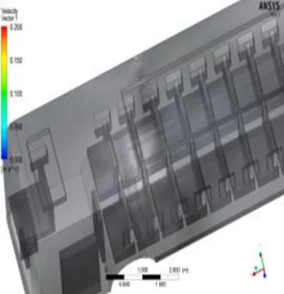
3) Vector plots: Vector flow is similar to streamline and shows the air flow through a particular region.

The input value for the bus is obtained after a lot of trial and error methods, when the inlet velocity is in the range of 1 &above , the back outlet pressure increases to the level of above 30m/s which was not feasible, therefore after running several trail and error the input values for the following was obtained .The velocities are higher in the middle section of the bus rather than in the front because there is an need of more reach. To achieve thermal comfort inside a bus , we need to do step by step analysis of the major factors involved , for maintaining a comfortable environment. This is an important factor , the speed of air entering the bus should be not too less and not too more , when the velocity of the air used is too high there is a lot of wastage of power and when the energy is too less , improper cooling is obtained. Therefore keeping the temp constant at 300k , we run multiple trial and error methods to obtain back outlet velocity.

Inl et s V e lo c it y1 V e lo c it y2 V e lo c it y3 V e lo c it y4 V e lo c it y T em p F ront i nl e t .04

.04 .04 .04 .04 300

S ide i n le t

.1 .15 .20 .25 .30 300

M iddl e i nl e t

.04 .04 .04 .04 .04 300

T

op

-m

idd

le

.09 .09 .09 .09 .09 300

Ba

c

k

2.341 2.519 2.746 2.9579 3.1738 300

This is the set of values that we obtain after ,multiple runs, keeping the all the inlet velocity constant other than the side inlet velocity , and obtain an average value..We choose the velocity set with the average value of back outlet velocity= 2.746m/s. The results from that case is explained below.

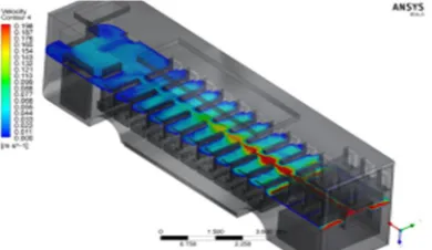
figure 3.4 contour plot on the (x-y) plane ,velocity

Figure 3.5 Contour Plot On The (Y-Z) Plane ,Velocity

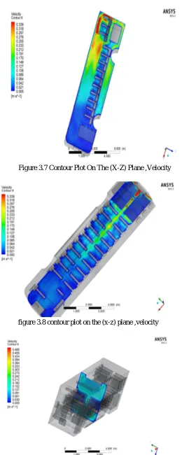
Figure 3.7 Contour Plot On The (X-Z) Plane ,Velocity

figure 3.8 contour plot on the (x-z) plane ,velocity

Figure 3.10 Contour Plot On The (X-Y) Plane ,Velocity

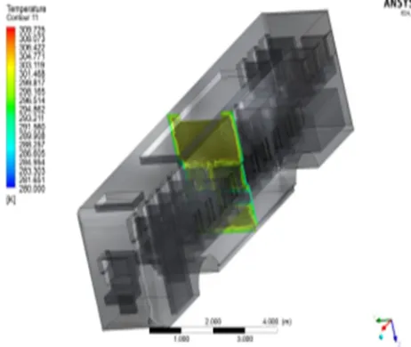
figure 3.11 contour plot on the (x-z) plane ,temperatu

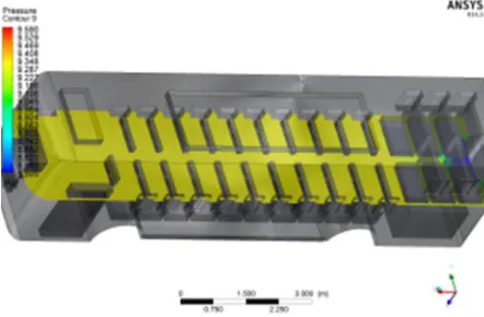
Figure 3.12 Contour Plot On The (Y-Z) Plane ,Pressure

Figure 3.14 Vector Plot

4) Summer Condition: We have to check the affect of velocity on each and every component of the bus with respect to the temperature change , first we take case of summer , during the case of summer the following are the average temperatures of the bus components

Components Temperature(summer) in K

seats 303

window 308

walls of buses 313

bottom of bus 315

roof top 318

Engine 473

Door 309

Gearbox 390

TABLE 3.2

These values are inputted for analysis along with the values obtained from table 3.1, the temperatures at the input are varied and the cooling effect is checked. Five different temperatures are checked and iteration is done, the completed results shows us the cooling effect produced at various inlet temperatures during summer.

Temp inlet Front vel Side vel Top vel Top-middle vel Back vel Outlet temp

284 .04 .20 .04 .09 2.6859 294.164

286 .04 .20 .04 .09 2.6859 295.4418

290 .04 .20 .04 .09 2.6859 298.07721

294 .04 .20 .04 .09 2.6859 300.459

296 .04 .20 .04 .09 2.6859 301.83

TABLE 3.3

We have received these values after putting everything for iteration ,the iteration at these varying temperatures at constant velocity tells us about the cooling effect produced at various temperatures by the system , we choose one of the results and explain it through plots & reports.

Figure 3.16 Contour Plot On The (Y-Z) Plane ,Velocity

Figure 3.17 Contour Plot On The (Y-X) Plane ,Velocity

Figure 3.18 Contour Plot On The (X-Z) Plane ,Velocity

Figure 3.20 Contour Plot On The (X-Y) Plane ,Velocity

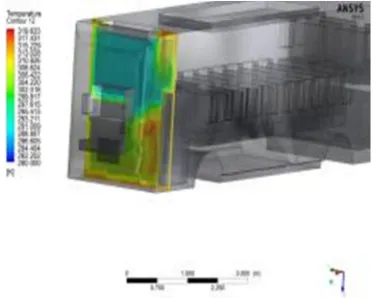
Figure 3.21 Contour Plot On The (Y-Z) Plane ,Temperature

Figure 3.23 Contour Plot On The (Y-Z) Plane ,Temperature

Figure 3.24 Contour Plot On The (X-Y) Plane , Temperature

Figure 3.26 Contour Plot On The (Y-Z) Plane ,Pressure

Figure 3.27 Contour Plot On The (X-Y) Plane ,Pressure

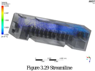
Figure 3.29 Streamiline

5) Winter Condition: Similar process is carried out by giving the temperatures of the winter condition , the value given are as below

Components Temperature(winter) in K

Seats 291

Window 290

walls of buses 293

bottom of bus 295

roof top 296

Engine 473

Door 289

Gearbox 390

. Table 3.4

T em p inl e t F ront v e l S ide ve l T op ve l T op -m idd le v e l Ba c k v e l O ut le t te m p

290 .04 .20 .04 .09 2.74 295.58

292 .04 .20 .04 .09 2.74 298.70

29

300 .04 .20 .04 .09 2.74 301.93

302 .04 .20 .04 .09 2.74 303.18

Table 3.5

We have received these values after putting everything for iteration ,the iteration at these varying temperatures at constant velocity tells us about the heating effect produced at various temperatures by the system , we choose one of the results and explain it through plots & reports.

Figure 3.30 Contour Plot On The (X-Y) Plane ,Velocity

Figure 3.31 Contour Plot On The (X-Z) Plane ,Velocity

Figure 3.33 Contour Plot On The (X-Y) Plane ,Velocity

Figure 3.34 Contour Plot On The (Y-Z) Plane ,Temperature

Figure 3.36 Contour Plot On The (Z-Y) Plane , Temperature

Figure 3.37 Contour Plot On The (X-Y) Plane , Temperature

Figure 3.40 Contour Plot On The (X-Z) Plane ,Pressure

6) Changing velocity, during summer & winter condition to check for variation in the effects We have seen the effects with same velocity , now to see that if there is a malfunction or slight change in the inlet velocity , what kind of change will be made in the effects produced.

For this we choose a temperature at which we have already conducted iteration, now we change the sidle inlet velocity to the values to see the effect.Summer at 290 K- velocity used at side inlets are 0.3 and 0.1 respectively. winter at 302 K- velocity used at side inlets are 0.3 and 0.1 respectively.

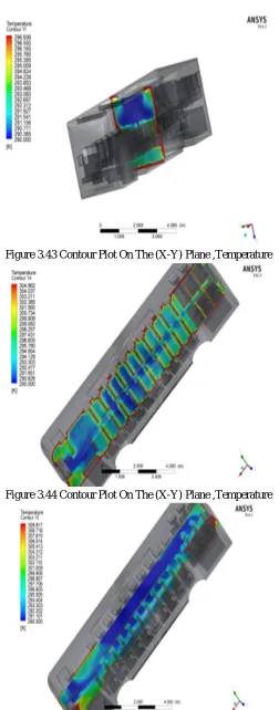
Figure 3.41 Contour Plot On The (X-Z) Plane ,Temperature

Figure 3.43 Contour Plot On The (X-Y) Plane ,Temperature

Figure 3.44 Contour Plot On The (X-Y) Plane ,Temperature

Figure 3.46 Contour Plot On The (Y-Z) Plane ,Temperature

Figure 3.47 Contour Plot On The (X-Z) Plane ,Temperature

Figure 3.49 Contour Plot On The (X-Y) Plane ,Temperature

Figure 3.50 Contour Plot On The (Z-Y) Plane, Temperature

Velocity/temp .03 .01

290(winter) 295 293

302(summer) 284 287

Table 3.6

Introduction of passengers in both the cases Till now we had been dealing with only the component of buses and now we add the final constraint of passengers.

Component Temperature in k

Passengers 310

now, we check this case of passengers at 2 conditions:we will check if the passenger are at thermal comfort , at maximum inlet temperature during summer i.e at 296 we will check if the passenger is at thermal comfort , at minimum inlet temperature during winter i.e at 290 K

Figure 3.51 Contour Plot On The (X-Y) Plane ,Velocity

Figure 3.52 Contour Plot On The (X-Z) Plane ,Velocity

Figure 3.54 Contour Plot On The (X-Z) Plane ,Velocity

Figure 3.55 Contour Plot On The (X-Y) Plane ,Velocity

Figure 3.57 Contour Plot On The (X-Z) Plane ,Velocity

Figure 3.58 Contour Plot On The (Y-Z) Plane ,Temperature

Figure 3.60 Contour Plot On The (X-Z) Plane ,Temperature

Figure 3.61 contour plot on the (y-z) plane ,temperature

Figure 3.62 Contour Plot On The (X-Z) Plane ,Temperature

Figure 3.65 Contour Plot On The (X-Y) Plane ,Velocity

Figure 3.66 Contour Plot On The (X-Y) Plane ,Velocity

Figure 3.67 Contour Plot On The (X-Z) Plane ,Velocity

Figure 3.69 Contour Plot On The (X-Z) Plane ,Velocity

Figure 3.70 Contour Plot On The (X-Y) Plane ,Temperature

Figure 3.72 Contour Plot On The (X-Z) Plane ,Temperature

Figure 3.73 Contour Plot On The (X-Y) Plane ,Temperature

Figure 3.74 Contour Plot On The (X-Y) Plane ,Pressure

Figure 3.76 Vector Plot

Weather/temperature Inlet temperature Obtained temperature range

Summer 296 292-295

Winter 290 291-295

Table 3.7

IV. CONCLUSIONS

A. The velocity we provide for air circulation is sufficient and reaches all the nook and corners of the bus providing proper thermal comfort with minimum energy being spent, the pressure and temperature of the component remaining constant.

B. The amount of air flow through each section is studies using streamlines vector plots and other graphs.

C. The same case is checked in the case of summer and winter seasons where the components of the bus and its parts are given average temperature corresponding to the season and the cooling or heating effect is studied successfully

D. The velocity is also varied for a particular temperature in both the seasons and the corresponding change in heating and cooling effect is recorded.

E. The passengers are added at last , and the effect corresponding to them and the whole bus is always carried out , we are able to find in both the cases that the passengers are able to experience thermal comfort with respect to the season change and the temperature.

REFERENCES

[1] Jalal M. Jalil and Haider Qassim Alwan,(2007) CFD Simulation for a Road Vehicle Cabin, JKAU: Eng. Sci., Vol. 18 No. 2, pp: 123-142.

[2] A. Alahmer, M.A. Omar, A. Mayyasb (2009), Effect of relative humidity and temperature control on in-cabin thermal comfort state: Thermodynamic and psychometric analyses, elsevier.com/locate/apthermeng.

[3] C.-H. CHIEN1, J.-Y. JANG1, Y.-H. CHEN (2008), 3-D NUMERICAL AND EXPERIMENTAL ANALYSIS FOR AIRFLOW WITHIN A PASSENGER COMPARTMENT, International Journal of Automotive Technology, Vol. 9, No. 4, pp. 437−445.

[4] Joo Hyun Moon, Jin Woon Lee, Chan Ho Jeong, Seong Hyuk Lee (2016)Thermal comfort analysis in a passenger compartment considering the solar radiation effect , International Journal of Thermal Sciences 107 (2016) 77e88

[5] Jan Pokorny, Jan Fiser, Miroslav Jicha(2014). Virtual Testing Stand for evaluation of car cabin indoor environment, Advances in Engineering Software 76 (2014) 48–55

[6] Boyd Roberto de Lieto Vollaro, (2013), Indoor climate analysis for urban mobility buses: a CFD model for the evaluation of thermal comfort, International Journal of Environmental Protection and Polic

[7] http://time.com/3942050/air-conditioner-healthy/, general survey of people in air conditioned environment