Multi-threaded Frequent Itemset Mining on
Temporal Data
PradnyaPatil1,Prof. N. R.Wankhade2
1, 2
Department of Computer Engineering Late G.N.Sapkal College Of Engineering, Nashik
Abstract: For analysis of transaction data, Frequent Itemset mining is important task in data mining. In literature work lot of work has been done on frequent Itemset mining task. But this work focuses on static dataset. Whole dataset is used for Itemset mining. The proposed work focuses on temporal data. Temporal data includes timestamp information. The dataset is sliced in cubes for analysis. The Apriori algorithm is used for Itemset mining. This data cube information provide periodic or time interval specific frequent Itemset. To define time cubes data density is defined to avoid overestimating the time period. To improve the system performance the system is implemented in multi-threaded environment. The performance of system will measured in terms of time and memory.
Keywords: apriori, multithreaded application, frequent Itemset, temporal data
I. INTRODUCTION
Extract interesting patterns form large dataset is important task in data mining. Transaction processing is important application in data mining. The transaction dataset like supermarket dataset contains the purchase records of different users. After analyzing the transaction dataset frequently sold items set can be extracted for e.g. bread with butter can be sold out frequently than break with Cadbury. For frequent itemset extraction, minimum support need to be defined first. The minimum support means the minimum number of transaction in which the itemset should present. It itemset satisfies the minimum support condition, then it is called as frequent itemset. For generating itemset, item purchase order is not considered.
Itemset retrieval is also called as co-occurrence pattern retrieval. This co-occurrence pattern retrieval technique was first proposed by Agrawal et al. [2]. There are various algorithms proposed in literature to mine frequent itemset such as: Apriori algorithm, Eclat Algorithm, FP-growth algorithm, etc. The apriori algorithm generates candidates form the dataset using download closure property and then finds frequent itemset based on support value. For dataset traversal it uses breadth-first search strategy. Eclat algorithm uses depth first search technique and set interaction theory. FP- growth algorithm generates tree structure using itemsets in a dataset. This algorithm does not generate the candidate itemset. For dataset traversal it uses tree traversal technique.
The frequent itemset mining can be applied in variety of domains such as: browsing link history, medical records, bank transaction history analysis, intrusion detection, continuous production, bioinformatics etc. In market basket analysis frequent itemset mining results helps to make a decision in marketing activities such as: product promotions, product placement, etc. All type of transaction data in a database is stored with timestamp entries. The record with time stamp entry is called as temporal record. The temporal aspect is one of the main dimensions of frequent itemset mining technique.
Different patterns can be discovered with the help of time information. Time specific pattern analysis can extracts useful knowledge form dataset such as: itemset purchase period, itemset highest purchase interval, lifespan of an item, etc.
Sequential association rules, time interval association rules, calendar specific interval rules are various frequent itemset mining technique based on temporal information.
In the following section various frequent itemset mining techniques are studied. These techniques use temporal information for frequent itemset extraction.
II. RELATED WORK
The first study related to the association rules discovery is presented by Agrawal et al.[2] in 1993. In this technique two things are focused: Finding frequent itemsets and generating association rules. This processing is done over purchase history of large items dataset. Unlike other statistical techniques, this technique considers Association rules are closely related to frequent itemset extraction.
technique extracts hourly daily, monthly , quarterly patterns. The pruning technique is applied to improve the performance of algorithm. The pattern can be called as cyclic pattern if it find in every cycle without any exception. This cyclic analysis helps in trend analysis and market forecasting. ramaswamy et al[4] proposes a new technique based on the technique proposed by Ozden et al. This technique uses user defined temporal patterns for rule discovery. The calendar algebra is used to process the time cycle. But this technique requires the prior knowledge of calendar data expression. In real life scenario, the product purchase history for defined cyclic period varies continuously. The product sold in one cycle may or may not be present in next cycle with same frequency. Hence the cyclic pattern discovery is not an appropriate solution for pattern discovery. To overcome this problem the periodic pattern discovery was proposed by Han et al. [5]. In this technique segment wise periodicity is defined with fixed length period. The periodicity based association rules extract good results for some time period but not for all. For temporal association rules extraction, Ale and Rossi[6] proposes a new technique. This technique stated that every item, itemset or rule have specific lifespan. This lifespan is defined in database. This technique extracts the association rules from a specific time period less than the database time period. This technique proposes a new concept called as: temporal support at the first time. Progressive-partition-miner[7] is proposed by Chang-Hung Lee and Ming-Syan Chen. This technique tried to focus on 2 problems: 1) Lack of exhibition period of each item and 2) lack of equitable support for each item. This technique initially portioned the database in light of exhibition periods of items. Afterwards it accumulates two-candidate based items occurrences progressively. The exhibition of period is same as the life span of an item presented in[6]. A generic algorithm is proposed by Matthews et al. [8] to find temporal association rules. This algorithm simultaneously searches the next rule in rule space and temporal space. This technique discovers more frequent itemsets over short time of interval of transaction dataset. This approach does not require prior partitioning. Xiao et al. [9] proposes a new technique for association rule discovery with time windows. This technique dynamically finds the time interval for association rule. No user defined interval is required. Here the length of interval is arbitrary. Saleh and Masseglia [10] finds the subset of dataset containing more frequent itemset. For e.g. items purchasing is more in Christmas than the summer. It dynamically determine the period by analyzing frequency of itemset. By traditional methods the itemset support might be less by considering the whole dataset. This technique is useful for seasonal product purchase behavior analysis. Mazaher Ghorbani and Masoud Abessi[1] proposes a new technique to mine frequent itemset over temporal data. This technique assumes that patterns are either hold in either some or all time intervals. This technique proposes a time cube analysis of frequent patterns. The whole dataset is divided in number of time cubes such as (hour, day, month), (day, month , year), etc. and analysis is done using apriori algorithm over these time cube data. It uses temporal support value concept. The processing is time consuming. The itemset should be mined for every time cube.
III. PROBLEM FORMULATION
Extraction of frequent Itemset from a transaction data is important task in data mining. The transaction entries vary periodically. Frequent Itemset mining need to be done based on temporal information. There is need to develop efficient time specific frequent Itemset extraction. Periodic or time interval specific frequent Itemset needs to be extracted from dataset.
IV. SYSTEM ARCHITECTURE
Following figure 1 shows the architecture of the system.
This system works on temporal data to mine frequent itemset. The data is sliced using temporal information. Data is divided in number of basic time cubes (BTC). The partitioning strategy is mentioned by user, It uses 3 level partitioning based on : (Hour, Day, Month), (Hour, Month, Year), (Day, Month, Year), etc. as per user input.
Dataset contains number of transactions. Each transaction contains number of items i, transaction unique identification number tid and timestamp information ts:
D={tid, <i1,i2,..in>, ts}
Initially, user mansions the time cube pattern for data slicing. Then the whole transaction dataset is partitioned according to the BTC cube. The frequent itemset mining algorithm is run for all BTC cube data.
Let N-cube be the number of transaction present in BTC time cube btc-k, X be the itemset present in btc-k and N(X)-cube be the number of transactions containing itemset X in btc-k. The support of itemset in btc-k is calculated as:
Support(X) = ( )
The minimum threshold is defined by the user. If itemset support is greater than the minimum support value then the itemset is called as frequent itemset.
The whole dataset is not equally distributed over time period. Hence after defining time cubes, data is unevenly partitioned in each time cube. Some data cube contains dense record set where as some data cube contains vary few records. The discovered itemset derived from few records may not find appropriate frequent itemset. So along with the support value density of data cube is also need to be defined.
The density of data cube represents, how densely the records present in the data cube by considering the whole dataset. Let N be the total number of records in a transaction dataset. And N-BTC is the number of time cubes generated as per the user BTC input parameter. The average number of records per cube can be calculated as:
A =
The α is the user predefined parameter. The value of α is lies in between 0 and 1. This parameter defined the desired density of data
cube. The density of cube is calculated as:
Density = α *A
For example, the total dataset contains 1000 records and as per the user requirement 10 BTC cubes are generated then the average records value is 100. Now if we define the value of α as 0. 5 then at least 50 records should be present in a given time cube.
Hence for frequent itemset data mining, following two conditions are important: Data cube must contain records equal or greater than the density value.
The itemset support value must be grater or equal to the predefined minimum threshold.
The apriory algorithm is used to find the frequent itemset from Time cubes. In apriory algorithm, initially large 1 itemset is calculated. Using Large 1 itemset candidates are generated. The candidates are again filtered using support value and minimum density value.
Discovering frequent itemset is time consuming. To find each item in transaction along with the Time cube information is time consuming task. To improve the system efficiency following two techniques are applied:
Hybrid data structure is used to store itemset information along with the time cube information. The transactions are stored in link list. Each link list store the hash table containing transaction timestamp as a key and itemset as a value. . To improve the candidate generation process the system uses multithreaded environment. The large 1 itemset is divided in two set to process individually. These threads find the candidate items and frequent itemset.
V. ALGORITHMS
A. Algorithm 1: mining Large1 itemsets
1) Input: Database -D, Minimum support-sup, Min density-den, Basic Time Cube-BTC
2) Output: Large 1 itemset L
3) Processing:
a) For all items in X
b) For all items in time cube D-BTC
Calculate support of X
c) For all BTC
e) Update Time cube TC with BTC
f) Add item X in large 1 itemset L
g) Else merge time cube with next time cube
h) Return L with TC
B. Algorithm 2: Candidate Generation 1) Input: Large 1 item set L
2) Output: Candidate items set C-set
3) Processing:
1) Generate items pairs in L as Li, Lj
2) For all pairs of L
3) Apply join operation over Li and Lj
4) If candidate length is K then
5) add candidate in C-set
6) return C-set
C. Algorithm 3: Mining Frequent Itemsets With Time Cubes
1) Input: Database -D, Minimum support-sup, Min density-den, Basic Time Cube-BTC
2) Output: Set of frequent itemsets F-set
3) Processing:
a) L: Call large 1 itemset algorithm to find itemset L with Time cube TC
b) Partition L in L1, L2 for parallel processing
c) For items in L1 and L2 generate 2 threads
d) C-set: Generate candidate for L1 and L2
e) For all itemset in C-set calculate support value in each TC
f) For all time Cubes
g) If support of itemset >= sup & density of TC > = den then
h) Add itemset in F-Set with TC information
i) Return F-set
VI. MATHEMATICAL MODEL
The system S can be defined as: S= {I, O, F} where
I = {I1, I2,I3,I4}, Set of Inputs I1 = Dataset
I2 = BTC parameters
I3 = Minimum Support Threshold I4= Minimum density Value O = {O1,O2} , Set of Outputs O1= Periodic frequent itemset O2 = Final Frequent itemset
F= {F1, F2, F3, F4, F5, F6, F7,F8} Set of Functions F1 = Upload dataset
VII. IMPLEMENTATION
A. Experimental Setup
The system is implemented using java with core i3 processor and 4 gb ram. For parallel data processing, Java multithreading programming is used to partition task among multiple threads.
B. Dataset
The transaction datasets - T10I4D100K , pumsb_star, Mushroom are downloaded from fimi site[11]. These dataset do not contain temporal information. To create temporal information user selects start and end date. From the interval of start and end date, a random date and time is created and assigned to the transaction. Based on the time information and time cube requirement data is portioned in multiple cubes.
C. Performance Metric
1) Number of itemset Extracted: The number of itemsets extracted from various BTC intervals are evaluated.
2) Time: The system performance of single threaded and multithreaded system is compared in terms of time.
3) Memory: The memory requirement for single threaded and multithreaded system is compared.
D. Results
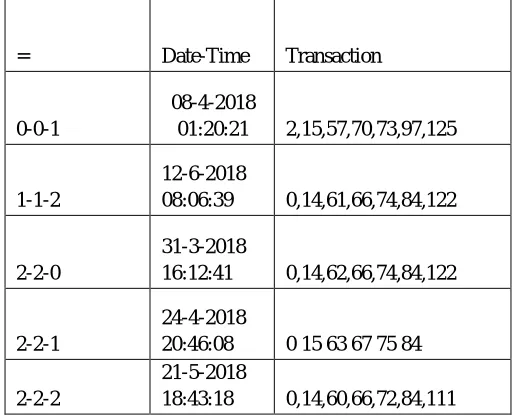
Following table I represent the sample of dataset with temporal information and time cube partitions. For dataset temporal partitioning, User selects start date and end date as an input along with the time cube information such as : (hour, date, month). With slot count 3, the whole data is portioned in 27 data cubes.
e.g: Start date: 17-03-2018 02:10:15 End Date: 27-06-2018 02:10:20 Slots Generated:
[image:5.612.177.433.446.655.2]Hour slot: 0.0-7.667, 7.667-15.334, 15.334-23.0 Date Slot: 1.0-11.0, 11.0-21.0, 21.0-31.0 Month Slot: 2.0-3.0, 3.0-4.0, 4.0-5.0
Table I: Sample dataset with temporal information and cube slicing
= Date-Time Transaction
0-0-1
08-4-2018
01:20:21 2,15,57,70,73,97,125
1-1-2
12-6-2018
08:06:39 0,14,61,66,74,84,122
2-2-0
31-3-2018
16:12:41 0,14,62,66,74,84,122
2-2-1
24-4-2018
20:46:08 0 15 63 67 75 84
2-2-2
21-5-2018
18:43:18 0,14,60,66,72,84,111
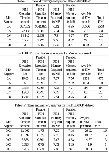
Table II: Time and memory analysis for Pumsb star dataset Min Support FIM Execution Time in seconds Parallel FIM Execution Time in seconds FIM Memory Required in MB Parallel FIM Memory required in MB Avg No of FIM per cube Total FIM
0.4 3076.72 3044.891 6.82 6.95 33506 9548
0.5 122.135 7.906 7.34 7.46 715 531
0.6 18.142 2.438 7.8 8.27 172 122
0.7 5.062 1.728 7.96 8.32 27 15
0.8 3 1.382 8.35 8.41 0.09 0
Table III: Time and memory analysis for Mashroom dataset
Min Support FIM Execution Time in Sec Parallel FIM Execution Time in Sec FIM Memory Required in MB Parallel FIM Memory required in MB Avg No of FIM per cube Total FIM
0.4 16.05 11.849 7.27 7.56 3358 675
0.5 5 2.093 7.3 7.62 1034 191
0.6 2.656 0.969 7.35 7.77 299 63
0.7 1.953 0.797 7.49 7.81 88 23
0.8 1.211 0.375 7.54 8.25 43 15
Table IV: Time and memory analysis for T40I10D100K dataset
Min Support FIM Execution Time in seconds Parallel FIM Execution Time in seconds FIM Memory Required in MB Parallel FIM Memory required in MB Avg No of FIM per cube Total FIM
0.04 12.062 1.75 7.25 7.48 26.42 16
0.05 11.097 0.922 7.55 8.45 10.57 5
0.06 6.858 0.891 7.67 8.63 4.57 3
0.07 5.626 0.75 7.72 8.65 1.9 1
0.08 3.205 0.734 7.88 8.8 0.33 0
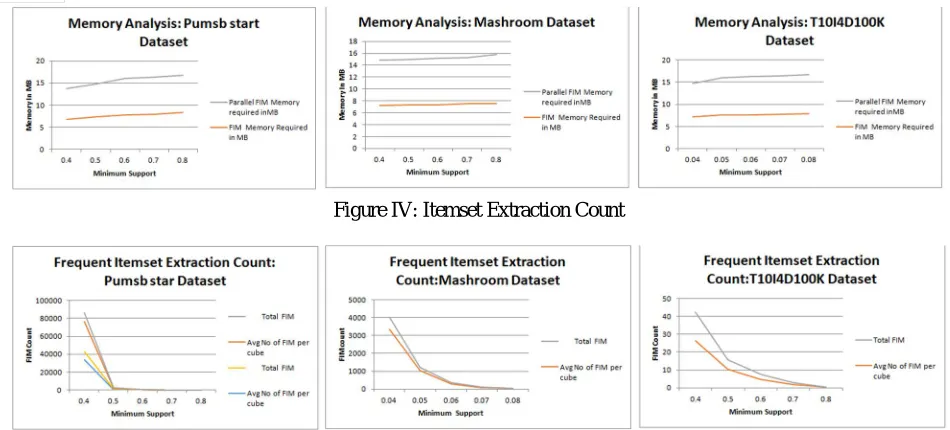
Following figure II and III shows the graphical representation of system comparison among single threaded and parallel threaded system processing in terms of time and memory for different datasets. Parallel processing requires less time as compared to the single thread application but it consumes little higher memory.
[image:6.612.61.554.636.714.2]Figure II: Time Analysis
Figure IV: Itemset Extraction Count
Figure IV represents the itemset extraction count. As minimum support value increases, the count of average number of frequent itemset extracted per cube and total itemset found over complete dataset decreases.
VIII. CONCLUSION
The system helps to find different frequent patterns over temporal dataset. The whole dataset is divided in time hierarchy using time data cubes. To mine valid patterns, a data cube density concept is proposed. Apriori algorithm is used to mine frequent itemset. To improve system efficiency multi-threaded environment is used with special data structure. The time required for processing dataset decreases with parallel thread execution. In future, The system can be implemented for continuous data stream.
REFERENCES
[1] Mazaher Ghorbani and Masoud Abessi, "A New Methodology for Mining Frequent Itemsets on Temporal Data", in IEEE Transactions on Engineering
Management, Vol. 64, Issue. 4, pp. 566 - 573, Nov 2017
[2] R. Agrawal, T. Imieli´nski, and A. Swami, “Mining association rules between sets of items in large databases,” ACM SIGMOD Rec., vol. 22, no. 2, pp. 207–
216, 1993.
[3] B.O zden, S. Ramaswamy, andA. Silberschatz, “Cyclic association rules,” in Proc. IEEE 14th Int. Conf. Data Eng., 1998, pp. 412–421.
[4] S. Ramaswamy, S. Mahajan, and A. Silberschatz, “On the discovery of interesting patterns in association rules,” in Proc. 24th Int. Conf. Very Large Data
Bases, 1998, pp. 368–379.
[5] J. Han, W. Gong, and Y. Yin, “Mining segment-wise periodic patterns in time-related databases,” in Proc. Int. Conf. Knowl. Discovery Data Mining, 1998, pp.
214–218.
[6] J. M. Ale and G. H. Rossi, “An approach to discovering temporal association rules,” in Proc. ACM Symp. Appl. Comput.-vol. 1, 2000, pp. 294–300.
[7] C.-H. Lee, M.-S. Chen, and C.-R. Lin, “Progressive partition miner: An efficient algorithm for mining general temporal association rules,” IEEE Trans. Knowl.
Data Eng., vol. 15, no. 4, pp. 1004–1017, Jul./Aug. 2003.
[8] S. G. Matthews, M. A. Gongora, and A. A. Hopgood, “Evolving temporal association rules with genetic algorithms,” in Research and Development in
Intelligent Systems XXVII. New York, NY, USA: Springer, 2011, pp. 107–120.
[9] Y. Xiao, R. Zhang, and I. Kaku, “A new framework of mining association rules with time-windows on real-time transaction database,” Int. J. Innov. Comput.,
Inf. Control, vol. 7, no. 6, pp. 3239–3253, 2011.
[10] B. Saleh and F. Masseglia, “Discovering frequent behaviors: Time is an essential element of the context,” Knowl. Inf. Syst., vol. 28, no. 2, pp. 311–331, 2011.