Deterministic Part Of Speech Tagging With Finite State Transducers

(1)

Deterministic Part-of-Speech Tagging

with Finite-State Transducers

Emmanuel Roche*

MERL

Yves Schabes*

MERL

Stochastic approaches to natural language processing have often been preferred to rule-based approaches because of their robustness and their automatic training capabilities. This was the case for part-of-speech tagging until Brill showed how state-of-the-art part-of-speech tagging can be achieved with a rule-based tagger by inferring rules from a training corpus. However, current implementations of the rule-based tagger run more slowly than previous approaches. In this paper, we present a finite-state tagger, inspired by the rule-based tagger, that operates in optimal time in the sense that the time to assign tags to a sentence corresponds to the time required to follow a single path in a deterministic finite-state machine. This result is achieved by encoding the application of the rules found in the tagger as a nondeterministic finite-state transducer and then turning it into a deterministic transducer. The resulting deterministic transducer yields a part-of-speech tagger whose speed is dominated by the access time of mass storage devices. We then generalize the techniques to the class of transformation-based systems.

1. Introduction

Finite-state devices have important applications to many areas of computer science, in- cluding pattern matching, databases, and compiler technology. Although their linguis- tic adequacy to natural language processing has been questioned in the past (Chomsky, 1964), there has recently been a dramatic renewal of interest in the application of finite- state devices to several aspects of natural language processing. This renewal of interest is due to the speed and compactness of finite-state representations. This efficiency is ex- plained by two properties: finite-state devices can be made deterministic, and they can be turned into a minimal form. Such representations have been successfully applied to different aspects of natural language processing, such as morphological analysis and generation (Karttunen, Kaplan, and Zaenen 1992; Clemenceau 1993), parsing (Roche 1993; Tapanainen and Voutilainen 1993), phonology (Laporte 1993; Kaplan and Kay 1994) and speech recognition (Pereira, Riley, and Sproat 1994). Although finite-state machines have been used for part-of-speech tagging (Tapanainen and Voutilainen 1993; Silberztein 1993), none of these approaches has the same flexibility as stochastic techniques. Unlike stochastic approaches to part-of-speech tagging (Church 1988; Kupiec 1992; Cutting et al. 1992; Merialdo 1990; DeRose 1988; Weischedel et al. 1993), up to now the knowledge found in finite-state taggers has been handcrafted and was not automatically acquired.

Recently, Brill (1992) described a rule-based tagger that performs as well as taggers based upon probabilistic models and overcomes the limitations common in rule-based approaches to language processing: it is robust and the rules are automatically ac-

(2)

Computational Linguistics Volume 21, Number 2

quired. In addition, the tagger requires drastically less space than stochastic taggers. However, current implementations of Brill's tagger are considerably slower than the

ones based on probabilistic models since it may require RKn elementary steps to tag

an input of n words with R rules requiring at most K tokens of context.

Although the speed of current part-of-speech taggers is acceptable for interac- tive systems where a sentence at a time is being processed, it is not adequate for applications where large bodies of text need to be tagged, such as in information re- trieval, indexing applications, and grammar-checking systems. Furthermore, the space required for part-of-speech taggers is also an issue in commercial personal computer applications such as grammar-checking systems. In addition, part-of-speech taggers are often being coupled with a syntactic analysis module. Usually these two modules are written in different frameworks, making it very difficult to integrate interactions between the two modules.

In this paper, we design a tagger that requires n steps to tag a sentence of length n, independently of the number of rules and the length of the context they require. The tagger is represented by a finite-state transducer, a framework that can also be the basis for syntactic analysis. This finite-state tagger will also be found useful when combined with other language components, since it can be naturally extended by composing it with finite-state transducers that could encode other aspects of natural language syntax.

Relying on algorithms and formal characterizations described in later sections, we explain how each rule in Brill's tagger can be viewed as a nondeterministic finite-state transducer. We also show how the application of all rules in Brill's tagger is achieved by composing each of these nondeterministic transducers and w h y nondeterminism arises in this transducer. We then prove the correctness of the general algorithm for determinizing (whenever possible) finite-state transducers, and we successfully apply this algorithm to the previously obtained nondeterministic transducer. The resulting deterministic transducer yields a part-of-speech tagger that operates in optimal time in the sense that the time to assign tags to a sentence corresponds to the time required to follow a single path in this deterministic finite-state machine. We also show how the lexicon used by the tagger can be optimally encoded using a finite-state machine. The techniques used for the construction of the finite-state tagger are then formalized and mathematically proven correct. We introduce a proof of soundness and completeness with a worst-case complexity analysis for the algorithm for determinizing finite-state transducers.

We conclude by proving that the method can be applied to the class of transformation- based error-driven systems.

2. Overview of Brill's Tagger

Brill's tagger is comprised of three parts, each of which is inferred from a training corpus: a lexical tagger, an unknown word tagger, and a contextual tagger. For purposes of exposition, we will postpone the discussion of the unknown word tagger and focus mainly on the contextual rule tagger, which is the core of the tagger.

The lexical tagger initially tags each word with its most likely tag, estimated by examining a large tagged corpus, without regard to context. For example, assuming that vbn is the most likely tag for the word "killed" and vbd for "shot," the lexical tagger might assign the following part-of-speech tags: 1

(3)

Emmanuel Roche and Yves Schabes Deterministic Part-of-Speech Tagging

Figure 1

Sample rules.

1. vbn vbd

PREVTAG

np

2. vbd vbn

NEXTTAG

by

(1) (2) (3)

Chapman/np killed/vbn John/np Lennon/np

John/np Lennon/np was/bedz shot/vbd by~by Chapman/np

He/pps witnessed/vbd Lennon/np killed/vbn by~by Chapman/np

Since the lexical tagger does not use a n y contextual information, m a n y words can be tagged incorrectly. For example, in (1), the w o r d "killed" is erroneously tagged as a verb in past participle form, and in (2), "shot" is incorrectly tagged as a verb in past tense.

Given the initial tagging obtained b y the lexical tagger, the contextual tagger applies a sequence of rules in order and attempts to r e m e d y the errors m a d e b y the initial tagging. For example, the rules in Figure 1 might be f o u n d in a contextual tagger.

The first rule says to change tag

vbn

to

vbd

if the previous tag is

np.

The second rule says to change

vbd

to tag

vbn

if the next tag is

by.

Once the first rule is applied, the tag for "killed" in (1) and (3) is changed from

vbn

to

vbd

and the following tagged sentences are obtained:

(4)

(5) (6)

Chapman/np killed/vbd John/np Lennon/np

John/np Lennon/np was/bedz shot/vbd by~by Chapman/np

He/pps witnessed/vbd Lennon/np killed/vbd by~by Chapman/np

A n d once the second rule is applied, the tag for "shot" in (5) is changed from

vbd

to

vbn,

resulting in (8), a n d the tag for "killed" in (6) is changed back from

vbd

to

vbn,

resulting in (9):

(7) (8) (9)

Chapman/np killed/vbd John/np Lennon/np

John/np Lennon/np was~be& shot/vbn by~by Chapman/np

He/pps witnessed/vbd Lennon/np killed/vbn by~by Chapman/np

It is relevant to our following discussion to note that the application of the NEXT- TAG rule m u s t look ahead one token in the sentence before it can be applied, and that the application of two rules m a y perform a series of operations resulting in no net change. As we will see in the next section, these two aspects are the source of local n o n d e t e r m i n i s m in Brill's tagger.

The sequence of contextual rules is automatically inferred from a training corpus. A list of tagging errors (with their counts) is compiled b y comparing the o u t p u t of the lexical tagger to the correct part-of-speech assignment. Then, for each error, it is determined which instantiation of a set of rule templates results in the greatest error reduction. Then the set of n e w errors caused by applying the rule is c o m p u t e d a n d the process is repeated until the error reduction drops below a given threshold.

(4)

A B PREVTAG C

A B PREVIOR2OR3TAG C A B PREVIOR2TAG C A B NEXTIOR2TAG C A B NEXTTAG C

A B SURROUNDTAG C D A B NEXTBIGRAM C D A B PREVBIGRAM C D

change A to B if previous tag is C

change A to B if previous one or two or three tag is C change A to B if previous one or two tag is C

change A to B if next one or two tag is C change A to B if next tag is C

change A to B if surrounding tags are C and D change A to B if next bigram tag is C D change A to B if previous bigram tag is C D

Figure 2

Contextual rule templates.

iii iilD ] C [C IA [

IclclAI

ICIDIClClAI

I C ID lii iiI ii iiiil

IClCIAI

IClClAI

(1)

(2)

Figure 3

Partial matches of A B PREVBIGRAM C C on the input C D C C A.

(3)

Using the set of contextual rule templates shown in Figure 2, after training on the Brown Corpus, 280 contextual rules are obtained. The resulting rule-based tagger performs as well as state-of-the-art taggers based upon probabilistic models. It also overcomes the limitations common in rule-based approaches to language processing: it is robust, and the rules are automatically acquired. In addition, the tagger requires drastically less space than stochastic taggers. However, as we will see in the next section, Brill's tagger is inherently slow.

3. Complexity of Brill's Tagger

Once the lexical assignment is performed, in Brill's algorithm, each contextual rule acquired during the training phase is applied to each sentence to be tagged. For each individual rule, the algorithm scans the input from left to right while attempting to match the rule.

This simple algorithm is computationally inefficient for two reasons. The first rea- son for inefficiency is the fact that an individual rule is compared at each token of the input, regardless of the fact that some of the current tokens may have been previously examined when matching the same rule at a previous position. The algorithm treats each rule as a template of tags and slides it along the input, one word at a time. Consider, for example, the rule A B P R E V B I G R A M C C that changes tag A to tag B if the previous two tags are C.

When applied to the input CDCCA, the pattern CCA is compared three times to

the input, as shown in Figure 3. At each step no record of previous partial matches or mismatches is remembered. In this example, C is compared with the second input token D during the first and second steps, and therefore, the second step could have been skipped by remembering the comparisons from the first step. This method is similar to a naive pattern-matching algorithm.

(5)

in a change (6) that is undone by the second rule as shown in (9). The algorithm may therefore perform unnecessary computation.

In summary, Brill's algorithm for implementing the contextual tagger m a y require

RKn

elementary steps to tag an input of n words with R contextual rules requiring at most K tokens of context.

4. Construction of the Finite-State Tagger

We show how the function represented by each contextual rule can be represented as a nondeterministic finite-state transducer and how the sequential application of each contextual rule also corresponds to a nondeterministic finite-state transducer being the result of the composition of each individual transducer. We will then turn the nondeterministic transducer into a deterministic transducer. The resulting part- of-speech tagger operates in linear time independent of the number of rules and the length of the context. The new tagger operates in optimal time in the sense that the time to assign tags to a sentence corresponds to the time required to follow a single path in the resulting deterministic finite-state machine.

Our work relies on two central notions: the notion of a finite-state transducer and the notion of a subsequential transducer. Informally speaking, a finite-state transducer is a finite-state automaton whose transitions are labeled by pairs of symbols. The first symbol is the input and the second is the output. Applying a finite-state transducer to an input consists of following a path according to the input symbols while storing the output symbols, the result being the sequence of output symbols stored. Section 8.1 formally defines the notion of transducer.

Finite-state transducers can be composed, intersected, merged with the union operation and sometimes determinized. Basically, one can manipulate finite-state transducers as easily as finite-state automata. However, whereas every finite-state automaton is equivalent to some deterministic finite-state automaton, there are finite-state transducers that are not equivalent to any deterministic finite-state transducer. Trans- ductions that can be computed by some deterministic finite-state transducer are called

subsequential functions.

We will see that the final step of the compilation of our tagger consists of transforming a finite-state transducer into an equivalent subsequential transducer.

We will use the following notation when pictorially describing a finite-state transducer: final states are depicted with two concentric circles; e represents the empty string; on a transition from state i to state j,

a/b

indicates a transition on input symbol a and output symbol(s) b; a a question mark (?) on an input transition (for example labeled

?/b)

originating at state i stands for any input symbol that does not appear as input symbol on any other outgoing arc from i. In this document, each depicted finite- state transducer will be assumed to have a single initial state, namely the leftmost state (usually labeled 0).

We are now ready to construct the tagger. Given a set of rules, the tagger is constructed in four steps.

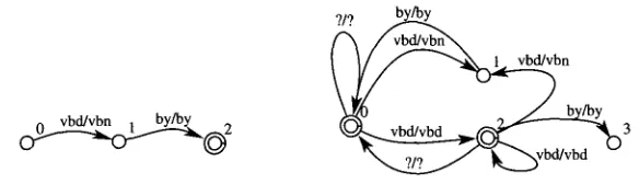
The first step consists of turning each contextual rule found in Brill's tagger into a finite-state transducer. Following the example discussed in Section 2, the functionality of the rule

vbn vbd PREVTAG np

is represented by the transducer shown on the left of Figure 4.

(6)

np/np vbn/vbd

[image:6.468.103.395.231.315.2]

?/? (.~p/np

Figure 4

Left: Transducer T1 representing the contextual rule vbn vbd PREVTAG np. Right: Local extension LocExt(T1) of T1.

bn

F i g u r e 5

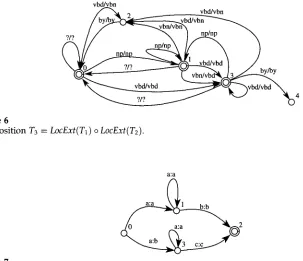
Left: Transducer T2 representing vbd vbn NEXTTAG by. Right: Local extension LocExt(T2) of T2.

Each contextual rule is defined locally; that is, the transformation it describes m u s t be applied at each position of the input sequence. For instance, the rule

A B PREVIOR2TAG C,

which changes A into B if the previous tag or the one before is C, m u s t be applied twice on C A A (resulting in the o u t p u t C B B). As we have seen in the previous section, this m e t h o d is not efficient.

The second step consists of turning the transducers p r o d u c e d b y the preceding step into transducers that operate globally on the input in one pass. This transformation is performed for each transducer associated with each rule. Given a function fl that transforms, say, a into b (i.e. fl(a) = b), we w a n t to extend it to a function f2 such that f2(w) = w / where w' is the w o r d built from the w o r d w where each occurrence of a has been replaced b y b. We say that f2 is the local extension 3 of fl, a n d we write f2 = LocExt(fl). Section 8.2 formally defines this notion a n d gives an algorithm for c o m p u t i n g the local extension.

Referring to the example of Section 2, the local extension of the transducer for the rule vbn vbd PREVTAG np is s h o w n to the right of Figure 4. Similarly, the transducer for the contextual rule vbd vbn NEXTTAG by a n d its local extension are s h o w n in Figure 5. The transducers obtained in the previous step still need to be applied one after the other.

(7)

vbd/vbn

[image:7.468.63.366.62.323.2]

~

4

Figure 6

Composition T3 = LocExt(T1) o LocExt(T2).

a : a

Figure 7

Example of a transducer not equivalent to any subsequential transducer.

The third step combines all transducers into one single transducer. This corresponds to the formal operation of composition defined on transducers. The formalization of this notion and an algorithm for computing the composed transducer are well known and are described originally by Elgot and Mezei (1965).

Returning to our running example of Section 2, the transducer obtained by composing the local extension of T2 (right in Figure 5) with the local extension of T1 (right in Figure 4) is shown in Figure 6.

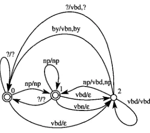
The fourth and final step consists of transforming the finite-state transducer obtained in the previous step into an equivalent subsequential (deterministic) transducer. The transducer obtained in the previous step may contain some nondeterminism. The fourth step tries to turn it into a deterministic machine. This determinization is not always possible for any given finite-state transducer. For example, the transducer shown in Figure 7 is not equivalent to any subsequential transducer. Intuitively speaking, this transducer has to look ahead an unbounded distance in order to correctly generate the output. This intuition will be formalized in Section 9.2.

However, as proven in Section 10, the rules inferred in Brill's tagger can always be turned into a deterministic machine. Section 9.1 describes an algorithm for determinizing finite-state transducers. This algorithm will not terminate when applied to transducers representing nonsubsequential functions.

(8)

Figure 8

Subsequential form for T3.

?/vbd,?

emits the empty symbol ¢, and postpones the emission of the output symbol. For

example, from the start state 0, the empty string is emitted on input

vbd,

while the

current state is set to 2. If the following word is

by,

the two token string

vbn by

is

emitted (from 2 to 0), otherwise

vbd

is emitted (depending on the input from 2 to 2 or

from 2 to 0).

Using an appropriate implementation for finite-state transducers (see Section 11), the resulting part-of-speech tagger operates in linear time, independently of the number of rules and the length of the context. The new tagger therefore operates in optimal time.

We have shown how the contextual rules can be implemented very efficiently. We n o w turn our attention to lexical assignment, the step that precedes the application of the contextual transducer. This step can also be made very efficient.

5. Lexical Tagger

The first step of the tagging process consists of looking up each word in a dictionary. Since the dictionary is the largest part of the tagger in terms of space, a compact representation is crucial. Moreover, the lookup process has to be very fast too---otherwise the improvement in speed of the contextual manipulations would be of little practical interest.

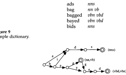
To achieve high speed for this procedure, the dictionary is represented by a deterministic finite-state automaton with both fast access and small storage space. Suppose one wants to encode the sample dictionary of Figure 9. The algorithm, as described by Revuz (1991), consists of first building a tree whose branches are labeled by letters and

whose leaves are labeled by a list of tags (such as

nn vb),

and then minimizing it into

a directed acyclic graph (DAG). The result of applying this procedure to the sample dictionary of Figure 9 is the DAG of Figure 10. When a dictionary is represented as a DAG, looking up a word in it consists simply of following one path in the DAG. The complexity of the lookup procedure depends only on the length of the word; in particular, it is independent of the size of the dictionary.

The lexicon used in our system encodes 54, 000 words. The corresponding DAG takes 360Kb of space and provides an access time of 12, 000 words per second. 4

[image:8.468.173.326.80.216.2]

(9)

ads nns

bag nn vb

bagged vbn vbd

bayed vbn vbd

[image:9.468.47.314.47.206.2]

bids nns

Figure 9

Sample dictionary.

a ~ " / d ~,O s ~ - ~ (nns)

_ ~ , / ~ 7 . ~ (nn,vb)

~-~O----~ ~) (vbd,vbn)

Figure 10

DAG representation of the dictionary of Figure 9.

6. Tagging Unknown Words

The rule-based system described by Brill (1992) contains a module that operates after all known words--that is, words listed in the dictionary--have been tagged with their most frequent tag, and before contextual rules are applied. This module guesses a tag for a word according to its suffix (e.g. a word with an "ing" suffix is likely to be a verb), its prefix (e.g. a word starting with an uppercase character is likely to be a proper noun), and other relevant properties.

This module basically follows the same techniques as the ones used to implement the lexicon. Because of the similarity of the methods used, we do not provide further details about this module.

7. Empirical Evaluation

The tagger we constructed has an accuracy identical s to Brill's tagger and comparable to statistical-based methods. However, it runs at a much higher speed. The tagger runs nearly ten times faster than the fastest of the other systems. Moreover, the finite- state tagger inherits from the rule-based system its compactness compared with a stochastic tagger. In fact, whereas stochastic taggers have to store word-tag, bigram, and trigram probabilities, the rule-based tagger and therefore the finite-state one only have to encode a small number of rules (between 200 and 300).

We empirically compared our tagger with Eric Brill's implementation of his tagger, and with our implementation of a trigram tagger adapted from the work of Church (1988) that we previously implemented for another purpose. We ran the three programs on large files and piped their output into a file. In the times reported, we included the time spent reading the input and writing the output. Figure 11 summarizes the results. All taggers were trained on a portion of the Brown corpus. The experiments were run on an HP720 with 32MB of memory. In order to conduct a fair comparison, the dictionary lookup part of the stochastic tagger has also been implemented using the techniques described in Section 5. All three taggers have approximately the same

(10)

Stochastic Tagger Speed 1,200 w / s

Space 2,158KB

Rule-Based Tagger 500 w / s

379KB

Finite-State Tagger 10,800 w / s

815KB

Figure 11

Overall performance comparison.

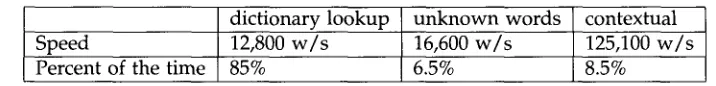
dictionary l o o k u p u n k n o w n w o r d s

Speed 12,800 w / s 16,600 w / s

Percent of the time 85% 6,5%

contextual 125,100 w / s 8.5%

Figure 12

Speeds of the different parts of the program.

precision (95% of the tags are correct). 6 By design, the finite-state tagger p r o d u c e s the same o u t p u t as the rule-based tagger. The rule-based t a g g e r - - a n d the finite-state t a g g e r - - d o not always p r o d u c e the exact same tagging as the stochastic tagger (they d o not m a k e the same errors); however, no significant difference in p e r f o r m a n c e b e t w e e n the systems was detected. 7

I n d e p e n d e n t l y , Cutting et aL (1992) q u o t e a p e r f o r m a n c e of 800 w o r d s per second for their part-of-speech tagger b a s e d on h i d d e n M a r k o v models.

The space required b y the finite-state tagger (815KB) is distributed as follows: 363KB for the dictionary, 440KB for the subsequential t r a n s d u c e r a n d 12KB for the m o d u l e for u n k n o w n words.

The speeds of the different parts of o u r system are s h o w n in Figure 12. 8

O u r system reaches a p e r f o r m a n c e level in s p e e d for w h i c h other, v e r y low-level factors (such as storage access) m a y d o m i n a t e the computation. At such speeds, the time s p e n t r e a d i n g the i n p u t file, breaking the file into sentences, breaking the sentences into w o r d s , a n d writing the result into a file is no longer negligible.

8. Finite-State Transducers

The m e t h o d s u s e d in the construction of the finite-state tagger described in the previous sections were described informally. In the following section, the notion of finite- state t r a n s d u c e r a n d the notion of local extension are defined. We also p r o v i d e an algorithm for c o m p u t i n g the local extension of a finite-state transducer. Issues related to the d e t e r m i n i z a t i o n of finite-state transducers are discussed in the section following this one.

8.1 Definition of Finite-State Transducers

A finite-state transducer T

is a five-tuple (~, Q,

i,F, E)

where: G is a f n i t e alphabet; Q is a finite set of states or vertices; i c Q is the initial state; F C Q is the set of final states; E c Q x (y, u {c}) x ~,* x Q is the set of edges or transitions.

6 For evaluation purposes, we randomly selected 90% of the Brown corpus for training purposes and 10% for testing.

7 An extended discussion of the precision of the rule-based tagger can be found in Brill (1992).

[image:10.468.82.405.49.88.2] [image:10.468.61.419.131.174.2]

(11)

1

Figure 13

T4: Example of a finite-state transducer.

For instance, Figure 13 is the graphical representation of the transducer:

T4 = (Ca, b,c,h,e}, C 0,1, 2,3}, o, {3}, C(0,a, b, 1), (0,a, c, 2), (1, h, h, 3), (2, e, e, 3)}).

A finite-state transducer T also defines a function on words in the following way: the extended set of edges F., the transitive closure of E, is defined by the following recursive relation:

• i f e E E t h e n e E / ~

• if (q,a,b,q'), (q',a',b',q") E E then (q, aa',bb',q") E E.

Then the function f from G* to ~* defined b y f ( w ) = w' iff 3q E F such that (i,w,w',q) E /~ is the function defined b y T. One says that T represents f and writes f = ITI. The functions on words that are represented b y finite-state transducers are called rational functions. If, for some input w, more than one o u t p u t is allowed (e.g. f(w) = {Wl, w2 . . . . }) then f is called a rational transduction.

In the example of Figure 13, IT41 is defined by IT4i(ah) = bh and IT4i(ae) = ce. Given a finite-state transducer T = (~, Q, i,F, E), the following additional notions are useful: its state transition function d that m a p s Q x (G u {¢}) into 2 Q defined b y d(q,a) = Cq' E Q I 3w' E G* and (q,a,w',q') E E}; and its emission function ~ that maps Q x (G u {~}) x Q into 2 ~" defined b y 6(q,a,q') = {w' E G* I (q,a,w,',q') E E}.

A finite-state transducer could be seen as a finite-state automaton, where each transition label is a pair. In this respect, T4 w o u l d be deterministic; however, since transducers are generally used to compute a function, a more relevant definition of determinism consists of saying that both the transition function d a n d the emission function ~ lead to sets containing at most one element, that is, Id(q,a)I < 1 a n d I~(q, a, qt)l < 1 (and that these sets are e m p t y for a = ~). With this notion, if a finite-state transducer is deterministic, one can apply the function to a given w o r d by determin- istically following a single path in the transducer. Deterministic transducers are called subsequential transducers (Schfitzenberger 1977). 9 Given a deterministic transducer, we can define the partial functions q®a = q' iff d(q,a) ~ {q~} and q,a = w ~ iff 3q' E Q such that q @ a = q~ and 6(q, a, q~) = Cw~}. This leads to the definition of subsequential trans- ducers: a subsequential transducer T' is a seven-tuple (G, Q,/, F, ®, *, p) where: ~, Q, i, F are defined as above; ® is the deterministic state transition function that maps Q x on Q, one writes q®a = q~; * is the deterministic emission function that m a p s Q x ~ on Y,*, one writes q • a = w~; a n d the final emission function p m a p s F on G*, one writes , ( q ) = w .

For instance, T4 is not deterministic because d(0,a) = C1,2}, but it is equivalent to T5 represented Figure 14 in the sense that they represent the same function, i.e.

(12)

Figure 14

Subsequential transducer T5.

h/bh 0 a& 1 , / " " - " ~ 2

b,c

Figure 15

T6: a finite-state transducer to be extended.

a a b c a b

b c b c

[image:12.468.47.300.48.289.2]

a a b c a b d c a

Figure 16

Top: Input. Middle: First factorization. Bottom: Second factorization.

IT4] = ] T s [ . T5 is d e f i n e d b y T5 = ( { a , b , c , h , e } , ( O , 1 , 2 } , O , { 2 } , ® , , , p ) w h e r e 0 ® a = 1, 0 , a = ¢, 1 ® h = 2, 1 , h = bh, 1 @ e = 2, 1 , e = ce, a n d p(2) = ~.

8.2 L o c a l E x t e n s i o n

In this section, w e will see h o w a function that n e e d s to be a p p l i e d at all i n p u t positions can be t r a n s f o r m e d into a global function that n e e d s to b e a p p l i e d once o n the input. For instance, consider T6 of Figure 15. It r e p r e s e n t s the function f6 = ]T6[ s u c h that f6(ab) = bc a n d f6(bca) = dca. We w a n t to build the function that, g i v e n a w o r d w, e a c h t i m e w contains ab (i.e. ab is a factor of the w o r d ) (resp. bca), this factor is t r a n s f o r m e d into its i m a g e bc (resp. dca). S u p p o s e , for instance, that the i n p u t w o r d is w = aabcab, as s h o w n in Figure 16, a n d that the factors that are in dom(f6) 1° c a n b e f o u n d a c c o r d i n g to t w o different factorizations: i.e. w I = a . w 2 . c-W211, w h e r e w2 -- ab, a n d wl = aa • w3 • b, w h e r e w3 = bca. T h e local extension of f6 will b e the t r a n s d u c t i o n that takes e a c h possible factorization a n d t r a n s f o r m s each factor a c c o r d i n g to f6, i.e. f6(w2) = bc a n d f6(w3) -= dca, a n d leaves the o t h e r p a r t s u n c h a n g e d ; h e r e this leads to t w o o u t p u t s : abccbc a c c o r d i n g to the first factorization, a n d aadcab a c c o r d i n g to the s e c o n d factorization.

T h e notion of local extension is f o r m a l i z e d t h r o u g h the following definition.

D e f i n i t i o n

If f is a rational t r a n s d u c t i o n f r o m G* to G*, the local extension F = LocExt(f) is the rational t r a n s d u c t i o n f r o m G* o n G* d e f i n e d in the following w a y : if u =

• ' ' . ' F ( u ) if E ~* •

a l b l a 2 b 2 • "anbnan+l E G* t h e n v = a l b l a 2 b 2 • "anbnan+l E ai - ( G *

dom(f) . ~*), bi c dom(f) a n d b I c f(bi).

(13)

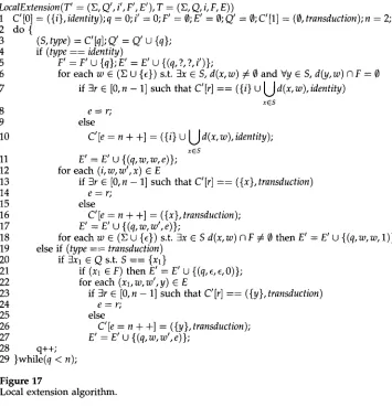
Local Extension ( T' = (G, Q', i', F', E' ) , T = (~., Q, i, F, E ) )

1 C'[0] = ({i}, identity); q = 0; i' = 0; F' = O; E' = 0; Q' = 0; C'[1] = (0, transduction); n = 2; 2 d o {

3 (S, type)= C'[q];Q' = Q ' u {q}; 4 if (type = = identity)

5 F' = F ' U {q};E' = E' u {(q, ?, ?, i')};

6 for each w E (~. U {¢}) s.t. 3x E S, d(x,w) # 0 and Vy E S, d(y,w) NF = O

7 if 3r E [0,n - 1] such that C'[r] = = ({i} U Ud(x,w),identity)

xES

8 e = r ;

9 else

10 C'[e = n + +] = ({i} U Ud(x,w),identity);

xES

11 E' = E' U {(q,w,w,e)};

12 for each (i, w, w', x) E E

13 if 3r E [0, n - 1] such that C'[r] = = ({x}, transduction)

14 e = r ;

15 else

16 C'[e = n + +] = ({x}, transduction);

17 E' = E' U {(q,w,w',e)};

18 for each w E (G U {c}) s.t. 3x E S d(x,w) MF # 0 then E' = E' U {(q,w,w, 1)};

19 else if (type = = transduction)

20 if 3Xl E Q s.t. S = = {Xl}

21 if (xi E F) then E' = E' U {(q,~,c,0)}; 22 for each (xl, w, w', y) E E

23 if 3r E [0, n -- 1] such that C'[r] = = ({y}, transduction)

24 e = r;

25 else

26 C'[e = n + +] = ({y}, transduction);

27 E' = E' U {(q,w,w',e)};

28 q++;

29 }while(q < n);

Figure 17

Local extension algorithm.

Intuitively, if F = LocExt(f) a n d w E ~*, e a c h f a c t o r o f w in dom(f) is t r a n s f o r m e d into its i m a g e b y f a n d the r e m a i n i n g p a r t o f w is left u n c h a n g e d . If f is r e p r e s e n t e d b y a finite-state t r a n s d u c e r T a n d LocExt(f) is r e p r e s e n t e d b y a finite-state t r a n s d u c e r T', o n e w r i t e s T' = LocExt(T).

It c o u l d also be s e e n t h a t if "YT is the i d e n t i t y f u n c t i o n o n •* - (~* • dom(T) • ~*),

t h e n LocExt(T) = "Tr " ( T . "yw)*. 12 F i g u r e 17 g i v e s a n a l g o r i t h m t h a t c o m p u t e s t h e local e x t e n s i o n directly.

T h e i d e a is t h a t a n i n p u t w o r d is p r o c e s s e d n o n d e t e r m i n i s t i c a l l y f r o m left to right. S u p p o s e , f o r instance, t h a t w e h a v e the initial t r a n s d u c e r T7 of F i g u r e 18 a n d t h a t w e w a n t to b u i l d its local e x t e n s i o n , Ts of F i g u r e 19.

W h e n the i n p u t is read, if a c u r r e n t i n p u t letter c a n n o t be t r a n s f o r m e d at t h e initial state o f T7 (the letter c for instance), it is left u n c h a n g e d : this is e x p r e s s e d b y t h e l o o p i n g t r a n s i t i o n o n the initial state 0 o f Ts l a b e l e d ?/?.13 O n t h e o t h e r h a n d ,

12 In this last f o r m u l a , the c o n c a t e n a t i o n • s t a n d s for the concatenation of the g r a p h s of each function; that is, for the c o n c a t e n a t i o n of the t r a n s d u c e r s v i e w e d as a u t o m a t a w h o s e labels are of the f o r m a/b. 13 A s e x p l a i n e d before, a n i n p u t transition labeled b y the s y m b o l ? s t a n d s for all t r a n s i t i o n s labeled w i t h

[image:13.468.37.392.60.429.2]

(14)

b,c

Figure 18

Sample transducer T7.

F.dE

?/?

[image:14.468.115.359.53.318.2]

Figure 19

Local extension Ts of TT: T8 =

LocExt(T7).

if the i n p u t symbol, say a, can be processed at the initial state of T7, one d o e s n ' t k n o w yet w h e t h e r a will be the b e g i n n i n g of a w o r d that can be t r a n s f o r m e d (e.g.

ab)

or w h e t h e r it will be followed b y a sequence that m a k e s it impossible to a p p l y the t r a n s f o r m a t i o n (e.g.

ac).

H e n c e one has to entertain t w o possibilities, n a m e l y (1) w e are processing the i n p u t according to T7 a n d the transitions s h o u l d be

a/b;

or (2) w e are w i t h i n the identity a n d the transition s h o u l d be

a/a.

This leads to two kind of states: the t r a n s d u c t i o n states ( m a r k e d

transduction

in the algorithm) a n d the identity states ( m a r k e d

identity

in the algorithm). It can be seen in Figure 19 that this leads to a t r a n s d u c e r that has a c o p y of the initial t r a n s d u c e r a n d an additional part that processes the identity while m a k i n g sure it could not h a v e b e e n transformed. In other words, the algorithm consists of building a c o p y of the original t r a n s d u c e r a n d at the same time the identity function that operates on ~* - ~* •

dom(T) • Y,.*

Let us n o w see h o w the algorithm of Figure 17 applies step b y step to the trans- d u c e r T7 of Figure 18, p r o d u c i n g the t r a n s d u c e r T8 of Figure 19.

In Figure 17, C'[0] = ({i},

identity)

of line 1 states that state 0 of the t r a n s d u c e r to be built is of type

identity

a n d refers to the initial state i = 0 of T7. q represents the current state a n d n the current n u m b e r of states. In the loop

do{...} while

(q < n), one builds the transitions of each state one after the other: if the transition points to a state not already built, a n e w state is a d d e d , thus i n c r e m e n t i n g n. The p r o g r a m stops w h e n all states h a v e b e e n inspected a n d w h e n no additional state is created. The n u m b e r of iterations is b o u n d e d b y 2 Ilz]l*2, w h e r e [[T[I = [Q[ is the n u m b e r of states of the original transducer. 14 Line 3 says that the current state w i t h i n the loop is q a n d that this state

(15)

1

[image:15.468.76.380.54.299.2]

?/?

Figure 20

Local extension T9 of T6:T9 =

LocExt(T6).

refers to the set of states S a n d is m a r k e d b y the t y p e

type.

In o u r e x a m p l e , at the first occurrence of this line, S is instantiated to {0} a n d

type = identity.

Line 5 a d d s the c u r r e n t identity state to the set of final states a n d a transition to the initial state for all letters that do n o t a p p e a r on a n y o u t g o i n g arc f r o m this state. Lines 6-11 build the transitions f r o m a n d to the identity states, k e e p i n g track of w h e r e this leads in the original transducer. For instance, a is a label that verifies the conditions of line 6. T h u s a transition

a/a

is to be a d d e d to the

identity

state 2, w h i c h refers to 1 (because of the transition

a/b

of T7) a n d to i = 0 (because it is possible to start the t r a n s d u c t i o n T7 f r o m a n y identity state). Line 7 checks that this state d o e s n ' t a l r e a d y exist a n d a d d s it if necessary, e = n + + m e a n s that the arrival state for this transition, i.e.

d(q,

w), will be the last a d d e d state a n d that the n u m b e r of states b e i n g built has to be i n c r e m e n t e d . Line 11 actually builds the transition b e t w e e n 0 a n d e = 2 labeled

a/a.

Lines 12-17 describe the fact that it is possible to start a t r a n s d u c t i o n f r o m a n y

identity

state. H e r e a transition is a d d e d to a n e w state, i.e.

a/b

to 3. The next state to be c o n s i d e r e d is 2 a n d it is built like state 0, except that the s y m b o l b s h o u l d block the c u r r e n t o u t p u t . In fact, state 1 m e a n s that w e a l r e a d y r e a d a w i t h a as o u t p u t ; thus, if one reads b,

ab

is at the c u r r e n t point, a n d since

ab

s h o u l d be t r a n s f o r m e d into

bc,

the c u r r e n t identity t r a n s f o r m a t i o n (that is a ~ a) s h o u l d be blocked: this is e x p r e s s e d b y the transition

b/b

that leads to state 1 (this state is a " t r a s h " state; that is, it has no o u t g o i n g transition a n d it is not final).

The following state is 3, w h i c h is m a r k e d as b e i n g of t y p e

transduction,

w h i c h m e a n s that lines 19-27 s h o u l d be applied. This consists s i m p l y of c o p y i n g the transitions of the original transducer. If the original state w a s final, as for 4 = ({2},

transduction),

an ~/~ transition to the initial state is a d d e d (to get the b e h a v i o r of T+).

(16)

9. Determinization

The basic idea b e h i n d the d e t e r m i n i z a t i o n a l g o r i t h m c o m e s f r o m M e h r y a r Mohri. is In this section, after giving a f o r m a l i z a t i o n of the algorithm, w e i n t r o d u c e a p r o o f of s o u n d n e s s a n d c o m p l e t e n e s s , a n d w e s t u d y its w o r s t - c a s e complexity.

9.1 Determinization Algorithm

In the following, for Wl, w 2 E

Y~,*,

Wl /~ W2 d e n o t e s the l o n g e s t c o m m o n prefix of wl a n d w2.

The finite-state t r a n s d u c e r s w e u s e in o u r s y s t e m h a v e the p r o p e r t y that t h e y can b e m a d e deterministic; that is, there exists a s u b s e q u e n t i a l t r a n s d u c e r that r e p r e s e n t s the s a m e function. 16 If T = (~, Q, i, F, E) is s u c h a finite-state transducer, the s u b s e q u e n t i a l t r a n s d u c e r T' = (E, Q', i', F', ®, ,, p) d e f i n e d as follows will be later p r o v e d e q u i v a l e n t to T:

Q~ c 2 QxE* . In fact, the d e t e r m i n i z a t i o n of the t r a n s d u c e r is related to the d e t e r m i n i z a t i o n of FSAs in the sense that it also i n v o l v e s a p o w e r set construction. T h e difference is that o n e h a s to k e e p track of the set of states of the original transducer, o n e m i g h t be in a n d also of the w o r d s w h o s e e m i s s i o n h a v e b e e n p o s t p o n e d . For instance, a state

{(ql, Wl), (q2,w2)} m e a n s that this state c o r r e s p o n d s to a p a t h that leads to q~ a n d q2 in the original t r a n s d u c e r a n d that the e m i s s i o n of wl (resp. w2) w a s d e l a y e d for ql (resp. q2).

i' = {(i, ~)}. T h e r e is no p o s t p o n e d e m i s s i o n at the initial state.

the e m i s s i o n function is d e f i n e d by:

S , a =

A

u.6(q,a,q')

(q,u)~S q' Ed(q,a)

This m e a n s that, for a g i v e n s y m b o l , the set of possible e m i s s i o n s is o b t a i n e d b y c o n c a t e n a t i n g the p o s t p o n e d e m i s s i o n s w i t h the e m i s s i o n at the c u r r e n t state. Since o n e w a n t s the transition to b e deterministic, the actual e m i s s i o n is the longest c o m m o n prefix of this set.

the state transition function is d e f i n e d by:

S ® a = U

U

{(q',(Sa)-l"u'6(q,a,q'))}*

(q,u)cS

q,~d(q,a)

G i v e n u, v E E*, u - v d e n o t e s the c o n c a t e n a t i o n of u a n d v a n d u -1 • v -- w, if w is s u c h that u - w -- v, u - I • v = 0 if n o s u c h w exists.

F ' = { S E Q ' I 3 ( q , u ) E S a n d q C F }

if

S E F t, p(S) = u

s.t. 3q E F, (q, u) C S. We will see in the p r o o f of correctness that p is p r o p e r l y defined.

15 Mohri (1994b) also gives a formalization of the algorithm.

(17)

The determinization algorithm of Figure 21 computes the above subsequential transducer.

Let us now apply the determinization algorithm of Figure 21 on the finite-state transducer T4 of Figure 13 and show how it builds the subsequential transducer T10 of Figure 22. Line 1 of the algorithm builds the first state and instantiates it with the pair {(0, e)}. q and n respectively denote the current state and the number of states having been built so far. At line 5, one takes all the possible input symbols w; here only a is possible, w' of line 6 is the output symbol,

w ' = e. ( A a(0,a,~')), ~'E{1,2}

thus w' = a(0,a, 1) A 6(0,a,2) = b A c = e. Line 8 is then computed as follows:

s'= U U

~ff{0} ~'E{1,2}

thus S' = { (1, a (0, a, 1 )) } U { (2, 6 (0, a, 2) } = { (1, b), (2, c) }. Since no r verifies the condition on line 9, a new state e is created to which the transition labeled a/w = a/e points and n is incremented. On line 15, the program goes to the construction of the transitions of state 1. On line 5, d and e are then two possible symbols. The first symbol, h, at line 6, is such that w' is

w' = A b. 6(1,h,~')) = bh. F/'cd(1,h)={2}

Henceforth, the computation of line 8 leads to

S'= U

U

{(q ''(bh)-l"b'h)}={(2"e)}"

qE{1} ~'E{2}

State 2 labeled {(2, e)} is thus added, and a transition labeled h/bh that points to state 2 is also added. The transition for the input symbol e is computed the same way.

The subsequential transducer generated by this algorithm could in turn be min- imized by an~'algorithm described in Mohri (1994a). However, in our case, the transducer is nearly minimal.

9.2 Proof of Correctness

Although it is decidable whether a function is subsequential or not (Choffrut 1977), the determinization algorithm described in the previous section does not terminate when run on a nonsubsequential function.

Two issues are addressed in this section. First, the proof of soundness: the fact that if the algorithm terminates, then the output transducer is deterministic and represents the same function. Second, the proof of completeness: the algorithm terminates in the case of subsequential functions.

Soundness and completeness are a consequence of the main proposition, which states that if a transducer T represents a subsequential function f, then the algorithm DeterminizeTransducer described in the previous section applied on T computes a sub- sequential transducer representing the same function.

(18)

Computational Linguistics Volume 21, N u m b e r 2

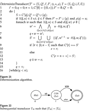
DeterminizeTransducer(T' = (G, Q ' , i', F', ®, , , p), T = (~I, Q, i, F, E))

9 10 11 12 13 14 15 16

i ' = 0;q = 0 ; n = 1;C'[0] = {(0,~)};F' = 0 ; Q ' = 0; d o {

S = C'[q];Q' = Q ' u {q};

if 3(~, u) ¢ S s.t. ~ ¢ F t h e n F' = F' U {q} a n d p(q) = u; f o r e a c h w s u c h t h a t 3(~,u) E S a n d d(~,w) • 0 {

w , =

A A

u 61,,w,,'l

G , ) e s ~'edGw) q * w = w ' ;

s ' =

U U

(~,u) es 7' edGw)

if 3r E [0,n -- 1] s u c h t h a t C'[r] = = S' e = r ;

else

C'[e = n + +] = S'; q @ w = e ;

}

q + + ; }while(q < n);

Figure 21

Determinization algorithm.

h/bh

Figure 22

Subsequential transducer T10 such that IT10I = IT4I .

t r a n s d u c e r s t h a t a r e r e d u c e d a n d t h a t are d e t e r m i n i s t i c in t h e s e n s e of finite-state a u t o m a t a . 17

I n o r d e r to p r o v e this p r o p o s i t i o n , w e n e e d to e s t a b l i s h s o m e p r e l i m i n a r y n o t a t i o n s a n d l e m m a s .

First w e e x t e n d t h e d e f i n i t i o n of t h e t r a n s i t i o n f u n c t i o n d, t h e e m i s s i o n f u n c t i o n 6, t h e d e t e r m i n i s t i c t r a n s i t i o n f u n c t i o n @, a n d the d e t e r m i n i s t i c e m i s s i o n f u n c t i o n * o n w o r d s in the classical way. W e t h e n h a v e the f o l l o w i n g p r o p e r t i e s :

ab) =

U

a(q',b)

6(ql,ab, q2) = U

6(ql, a,

q ' ) . 6(q', b,

q2)

{q' Cd(ql,a) [q2 Cd(q',b ) }

q ® a b = ( q ® a ) ® b

[image:18.468.48.344.53.424.2] [image:18.468.75.363.545.642.2]

(19)

q , a b = ( q , a ) . ( q ® a ) , b

For the following, it is useful to note that if IT I is a function, then 6 is a function too.

The following l e m m a states an invariant that holds for each state S built within the algorithm. The l e m m a will later be used for the p r o o f of soundness.

Lemma 1

Let I = C'[0] be the initial state. At each iteration of the " d o " loop in Determinize- Transducer, for each S --- C'[q] a n d for each w E ~* such that I ® w = S, the following holds:

(i)

I , w =

/~

6(i,w,q)

qEd(i,w)

(ii) S = I ® w = { ( q , u ) l q E d ( i , w ) a n d u = ( I * w ) - l . 6 ( i , w , q ) }

Proof

(i) and (ii) are o b v i o u s l y true for S = I (since d(i, ~) = i a n d ~(i, c, i) = c), a n d w e will s h o w that given some w E ~* if it is true for S = I ® w, then it is also true for $1 = S @ a = I Q wa for all a E Y..

A s s u m i n g that (i) a n d (ii) hold for S a n d w, then for each a E ~:

A

~(i,w,q). ~(q,a,q')

qEd(i,w),q' Ed(q,a)

= ( I , w ) .

A

')

qEd( i,w),q' Ed(q,a )

=

A

(q,u ) ES=I®w,q' Ed(q,a)

= ( I , w ) . ( S , a )

= I , w . ( I ® w ) , a

= I , w a

This p r o v e s (i).

We n o w turn to (ii). A s s u m i n g that (i) a n d (ii) hold for S a n d w, then for each a E ~, let $1 = S ® a; the algorithm (line 8) is such that

$1 = ( ( q ' , u ' ) ] 3 ( q , u ) E S , q ' E d(q,a) a n d u ' = ( S , a ) -1 . u . 6 ( q , a , q ' ) }

Let

$2 -- {(q',u') I q' E d(i, wa) and u' = (I • wa) - 1 . 6(i, wa, q')}

We s h o w that $1 c $2. Let (q',u') E $1, then 3 ( q , u ) E S s.t. q' E d(q,a) a n d u' = (S * a ) - l . u . 6(q, a, q'). Since u = (I • w ) - I . 6(i, w, q), then u' = (S * a ) - I . (I * w ) - I . 6 ( i , w , q ) . 6(q,a,q'); that is, u' = ( I * w a ) - 1 . 6(i, wa, q'). Thus (q',u') E $2. H e n c e $1 c $2. We n o w s h o w that $2 c $1. Let (q',u') E $2, a n d let q E d ( i , w ) be s.t. q' E d(q,a) a n d u = ( I , w ) -1 . 6 ( i , w , q ) then (q,u) E S and since u' = ( I * wa) -1 • 6(i, wa, q') =

( s , a ) - 1 • u . ( q ' , u ' ) E s l

(20)

The following l e m m a states a c o m m o n property of the state S, which will be used in the complexity analysis of the algorithm.

Lemma 2

Each S = C'[q] built within the "do" loop is s.t. Vq E Q, there is at most one pair (q, w) c S with q as first element.

Proof

Suppose (q, wl) c S a n d (q, w2) c S, a n d let w be s.t. I ® w = S. Then W l = ( I • W ) - 1 '

fi(i, w, q) a n d w2 = (I • w ) - I . 6(i, w, q). Thus W 1 = W 2. [ ]

The following l e m m a will also be used for soundness. It states that the final state emission function is indeed a function.

Lemma 3

For each S built in the algorithm, if (q, u), (q', u') c S, then q, q' E F ~ u = u'

Proof

Let S be one state set built in line 8 of the algorithm. Suppose (q, u), (q', u') E S a n d q, q' E F. According to (ii) of l e m m a 1, u = ( I , w ) -1 .6(i,w,q) a n d u' = ( I , w ) -1.6(i,w,q'). Since IT[ is a function a n d {6(i,w,q),6(i,w,q')} E ITl(w) then 6(i,w,q) = 6(i,w,q'), therefore u = uq []

The following l e m m a will be u s e d for completeness.

Lemma 4

Given a transducer T representing a subsequential function, there exists a b o u n d M s.t. for each S built at line 8, for each (q,u) E S, lu[ < M.

We rely on the following theorem proven by Choffrut (1978):

Theorem 1

A function f on G* is subsequential iff it has b o u n d e d variations a n d for a n y rational language L C ~*, f-1 (L) is also rational.

with the following two definitions:

Definition

The left distance between two strings u a n d v is I[u,v[I = [u[ + Iv[ - 2[u/~ v[.

Definition

A function f on G* has b o u n d e d variations iff for all k ~ 0, there exists K > 0 s.t. u,v C dom(f), [[u,v[[ <_ k ~ ][f(u),f(v)[[ <_ K.

Proof of Lemma 4

(21)

in T. For each q c Q let

s(q) E Q

be a state s.t.

s(q) c d(q,c(q)) AF.

Let us f u r t h e r define

M1 = maxl6(q,c(q),s(q))]

qEQ

M2

= m a x Ic(q)l

qEQ i %l~ l

Since f is subsequential, it is of b o u n d e d variations, therefore there exists K s.t. if ][u, vi] ~ a M 2 t h e n

I[f(u),f(v)] I G K.

Let M = K + 2M1.

Let S be a state set built at line 8, let w be s.t.

I ® w = S

a n d A =

I , w .

Let (ql, u) E S. Let (q2, v) C S be s.t. u A v = c. Such a pair a l w a y s exists, since if n o t

t h u s [A.

] A u'] > 0

(q',u')ES

A

u'l = I A

.x'u'l>l,',l

(q',u')~s

(q',u')cs

Thus, because of (ii) in L e m m a 1,

I A

6(i,w,q')]

> I I , w l

q' Ed(i,w)

w h i c h contradicts (i) in L e m m a 1.

Let w = ~(ql,

c(ql), s(ql))

a n d a;' = 6(q2, c(q2), s(q2)).

Moreover, for a n y

a,b,c,d E ~, Iia, ciI <_ ]lab, cd[I +*

Ibl + [d I. In fact,

Ilab, cdiI =

[ab[ + IcdI- 2Iab A cd I

= lal + I c] + IbI + I d I -

2Iab A cd I

= II a, c]I + 21a A c I + [b I + ]d I - 2 l a b

A cd I

b u t

labAcd] <_

laAcI +Ib[+]d[ a n d since

]Iab, cd[I

= Ila, cI[-2([abAcd

I -[aAc

I - [ b I -IdI) - IbI- IdI o n e has Iia, cil <

I]ab, cdll +

Ib[ + Idl.

Therefore, in particular, luI < ][Au, AvI[ <

JiAua;,Avw'][ +

]0; I + Iw'I, t h u s I u] < Iif(w •

c(ql)),f(w,

c(q2))I] q- 2M1. But ][w.

c(ql),W"

c(q2)ll G ]c(ql)[ + Ic(q2)I ~

2M2,

t h u s Iif(w •

c(ql)),f(w"

c(q2))[] < K a n d therefore I u] < K + 2M 1 = M. []

The time is n o w ripe for the m a i n proposition, w h i c h proves s o u n d n e s s a n d completeness.

Proposition

If a t r a n s d u c e r T represents a s u b s e q u e n t i a l f u n c t i o n f, t h e n the a l g o r i t h m

Determinize-

Transducer

described in the p r e v i o u s section a p p l i e d on T c o m p u t e s a s u b s e q u e n t i a l t r a n s d u c e r ~- r e p r e s e n t i n g the s a m e function.

Proof

L e m m a 4 s h o w s t h a t the a l g o r i t h m a l w a y s t e r m i n a t e s if IT] is subsequential.

Let us s h o w that

dom(iTI) c dom(iTI).

Let w E ~* s.t. w is n o t in

dom(iTI),

t h e n

d(i,

w) M F = 0. Thus, a c c o r d i n g to (ii) of L e m m a 1, for all (q, u) c I ® w, q is n o t in F, t h u s I ® w is n o t t e r m i n a l a n d therefore w is n o t in

dom(~-).

(22)

9.3 Worst-Case Complexity

In this section we give a worst-case u p p e r b o u n d of the size of the subsequential transducer in terms of the size of the input transducer.

Let L = {w E G" s.t. Iw[ <__ M}, where M is the b o u n d defined in the proof of L e m m a 4. Since, according to L e m m a 2, for each state set Q~, for each q E Q, Q' contains at most one pair (q, w), the maximal n u m b e r N of states built in the algorithm is smaller than the s u m of the n u m b e r of functions from states to strings in L for each state set, that is

N

<

ILl IQ't

Q' E2Q

we thus have N _< 2 IQI x ILl iQI -- 2 IQI x 2 [Qlxl°g2 iLl a n d therefore N _< 2 IQl(l+l°glLI). Moreover,

M + ' - 1

ILl

= 1 + lye] + . . . + ISl M - ISl - 1 i f I s ] > 1

a n d

ILl

= M + I if = 1. In this last formula, M = K + 2 M 1 , as described in L e m m a 4. Note that if P =

MAXa~sl6(q,a,

q')l is the maximal length of the simple transitions emissions, M1 ~ IQI x P, thus M _< K + 2 x IQI x P.

Therefore, if [E I > 1, the n u m b e r of states N is bounded:

i:gl(K+2 x IQI xP+1-1 )

N <_ 2 IQIx(l+l°g i~l-,

a n d if lee = 1,

N ~

2 [QIx(l+l°g(K+2xiQLxP+l))

10. Subsequentiality of Transformation-Based Systems

The proof of correctness of the determinization algorithm a n d the fact that the algorithm terminates on the transducer encoding Brill's tagger s h o w that the final function is subsequential a n d equivalent to Brill's original tagger.

In this section, we prove in general that a n y transformation-based system, such as those used by Brill, is a subsequential function. In other words, a n y transformation- based system can be t u r n e d into a deterministic finite-state transducer.

We define transformation-based systems as follows.

Definition

A transformation-based system is a finite sequence ( f ] , . . . , f n ) of subsequential functions w h o s e d o m a i n s are bounded.

A p p l y i n g a transformation-based system consists of applying each function

fi

one after the other. A p p l y i n g one function consists of looking for the first position in the input at which the function can be triggered. W h e n the function is triggered, the longest possible string starting at that position is transformed according to this function. After the string is transformed, the process is iterated starting at the end of the previously transformed string. Then, the next function is applied. The p r o g r a m ends w h e n all functions have been applied.

It is not true that, in general, the local extension of a subsequential function is subsequential. TM For instance, consider the function

fa

of Figure 23.

(23)

Figure 23

Function fa.

a:b a:b a:b

The local extension of the function fa is not a function. In fact, consider the i n p u t string daaaad; it can be d e c o m p o s e d either into d • aaa. ad or into da • aaa. d. The first d e c o m p o s i t i o n leads to the o u t p u t dbbbad, a n d the second o n e to the o u t p u t dabbbd.

The i n t e n d e d use of the rules in the tagger defined b y Brill is to a p p l y each function f r o m left to right. In addition, if several d e c o m p o s i t i o n s are possible, the o n e that occurs first is the o n e chosen. In o u r p r e v i o u s e x a m p l e , it m e a n s that o n l y the o u t p u t dbbbad is generated.

This notion is n o w d e f i n e d precisely.

Let a be the rational function d e f i n e d b y a(a) = a for a c ~, a([) = a(]) = ~ on the additional s y m b o l s '[' a n d ']', w i t h a such that a ( u . v) = a ( u ) . a(v).

Definition

Let Y c ~ + a n d X = ~* - ~*. Y. ~*, a Y - d e c o m p o s i t i o n of x is a string y E X. ([. Y. ]. X)* s.t. a(y) = x

For instance, if Y = dom(fa) -- {aaa}, the set of Y - d e c o m p o s i t i o n s of x = daaad is { d [aaa ]ad , da [aaa ] d }.

Definition

Let < be a total o r d e r on P, a n d let ~ = ~ U {[,]} be the al _phabet ~ w i t h the t w o additional s y m b o l s '[' a n d ']'. Let extend the o r d e r > to N b y Va E ~, ' [ ' < a a n d a < ']'. < defines a lexicographic o r d e r on ~* that w e also d e n o t e <. Let Y c 2 + a n d x c N*, the minimal Y-decomposition of x is the Y - d e c o m p o s i t i o n w h i c h is m i n i m a l in (~*, <).

For instance, the m i n i m a l dom(fa)-decomposition of daaaad is d[aaa]ad. In fact, d[aaaJad < da[aaa]d.

Proposition

G i v e n Y C ~ + finite, the function mdy that to each x c G* associates its m i n i m a l Y-decomposition, is s u b s e q u e n t i a l a n d total.

Proof

Let dec be defined b y dec(w) = u . [. v . 1. dec((uv) -1 . w), w h e r e u, v E P~* are s.t. v E Y, 3v' c ~* w i t h w = uvv' a n d lul is m i n i m a l a m o n g such strings a n d dec(w) -- w if no s u c h u, v exists. The function mdy is total b e c a u s e the function dec a l w a y s r e t u r n s an o u t p u t that is a Y - d e c o m p o s i t i o n of w.

We shall n o w p r o v e that the function is rational a n d t h e n that it has b o u n d e d variations; this will p r o v e a c c o r d i n g to T h e o r e m 1 that the function is subsequential. In the following X = ~* - P,* • Y- P,*. The t r a n s d u c t i o n Ty that g e n e r a t e s the set of Y - d e c o m p o s i t i o n s is d e f i n e d b y

Ty = I d x . ( e f t . I d y - c / ] . Idx)*

Deterministic Part Of Speech Tagging With Finite State Transducers