Advanced Computer Methods for Grounding
Analysis
Ignasi Colominas, Jos´e Par´ıs, Xes´us Nogueira, Ferm´ın Navarrina and Manuel Casteleiro
Abstract—We present a numerical formulation for grounding analysis that has been enterely developed by the authors within the last years. This approach is based on the Boundary Element Method and it has been implemented in a freeware application for the in-house computer aided design and analysis of ground-ing grids. The actual version of this software (TOTBEM) is already available for testing purposes (and also for its technical use) at no cost and can be run on any basic personal computer (as of 2012) with no special requirements. Furthermore, the scope and power of the proposed approach are shown by solving some important application problems in electrical engineering.
Index Terms—grounding, earthing analysis, boundary ele-ments, computer methods
I. INTRODUCTION
M
AIN goals of an earthing system are to safeguard that persons working or walking in the surroundings of the grounded installation are not exposed to dangerous electrical shocks and to guarantee the integrity of equipment and the continuity of the power supply under fault conditions. Thus, the equivalent resistance of the electrode should be low enough to assure the current dissipation mainly into the earth, while maximum potential differences between close points on the earth surface must be kept under certain maximum values defined by the safety regulations [1]–[3].Although the electric current dissipation is a well-known phenomenon, the analysis of a large electrical substation grounding in a practical case presents important difficulties that are mainly due to the specific geometry of the grid itself [4], [5]. The equations that govern the current dissipation into the soil through a grounded electrode are given by
div(σσσσσσσσσσσσσσ) = 0, σσσσσσσσσσσσσσ=−γγγγγγγγγγγγγγgrad(V)inE; σ
σ σσσσσ σ
σσσσσσtnnnnnnnnnnnnnnE= 0inΓE; V =VΓ inΓ; V →0, if|xxxxxxxxxxxxxx| → ∞(1)
whereEdenotes the earth,γγγγγγγγγγγγγγits conductivity,ΓEits surface,
n n nnnnn n
nnnnnnE its normal exterior unit field and Γ the surface of the
electrodes of the grounding grid [7]. The solution of this problem provides the current densityσσσσσσσσσσσσσσand the potential V at any pointxxxxxxxxxxxxxxwhen the grounded electrode is energized to a Ground Potential Rise (or GPR)VΓwith respect to remote
earth. Furthermore, most safety parameters that characterize an earthing system should be obtained straight from V computed on ΓE andσσσσσσσσσσσσσσonΓ [7], [9].
The selection of the appropriate soil model is an impor-tant issue in the definition of the mathematical model for
Manuscript received July 7, 2012; revised July 27, 2012. This work was supported in part by the Spanish “Ministerio de Educaci´on y Ciencia” under Grants DPI2009 14546-C02-01 and DPI2010-16496), by R&D projects of the Xunta de Galicia under Grants CN2011/002, PGDIT09 MDS00718PR and PGDIT09 REM005118PR and by FEDER funds.
The authors are with the Group of Numerical Methods in Engineering (GMNI) at the Civil Engineering School, University of A Coru˜na, SPAIN. Web page: http://caminos.udc.es/gmni, e-mail: [email protected]
[image:1.595.354.522.578.737.2]0 10 20 50 m
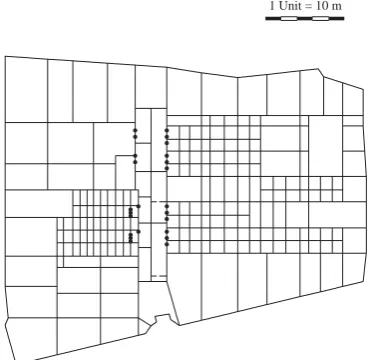
Fig. 1. Barber´a grounding system: grid plan.
grounding analysis: evidently, it is not feasible (or from an engineering point of view neither economic nor practical) to consider all variations of the soil conductivity. For this reason some soil models have been proposed, since the simplest, that is the isotropic and homogeneous one (“uniform soil model”) where an scalar conductivityγis introduced instead of conductivity tensorγγγγγγγγγγγγγγ [1], [7]; to the more complex, that is the “layered models” where the soil is represented in a number of strata, each one defined by means of a scalar conductivity and thickness [1].
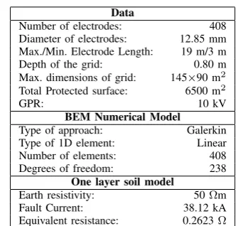
TABLE I
BARBERA´GROUNDINGSYSTEM: CHARACTERISTICS, NUMERICAL MODEL& RESULTS
Data
Number of electrodes: 408 Diameter of electrodes: 12.85 mm Max./Min. Electrode Length: 19 m/3 m Depth of the grid: 0.80 m Max. dimensions of grid: 145×90 m2 Total Protected surface: 6500 m2
GPR: 10 kV
BEM Numerical Model Type of approach: Galerkin Type of 1D element: Linear
Number of elements: 408
Degrees of freedom: 238
One layer soil model
Earth resistivity: 50Ωm
Fault Current: 38.12 kA
Equivalent resistance: 0.2623Ω
-20.00 0.00 20.00 40.00 60.00 80.00 100.00 -20.00
[image:2.595.54.286.51.369.2]0.00 20.00 40.00 60.00 80.00 100.00 120.00 140.00 160.00
Fig. 2. Barber´a grounding system: Potential distribution on the ground.
equation. This integral approach is the starting point for the development of a general numerical formulation based on the Boundary Element Method which allows to derive specific numerical algorithms of high accuracy for grounding analysis embedded in uniform soils models [7]. On the other hand, the anomalous asymptotic behaviour of the clasical computer methods proposed for earthing analyis can be rigorously explained identifying different sources of error [4]. Besides, the Boundary Element formulation has been extended for grounding grids embedded in stratified soils [8], [9]. Next, some examples of these models applied to the grounding analysis of several cases (by using real geometries of earthing electrodes) are presented; furthermore, it is shown the analysis of some very interesting related problems in electrical engineering practice.
II. GROUNDINGANALYSIS INUNIFORMSOILMODELS
[image:2.595.304.550.55.135.2]The first example corresponds to the grounding analysis of the Barber´a substation by using a uniform soil model. Figure 1 shows the plan of the grounding grid and the Table I summarizes the main characteristics of the earthing system, as well as, the numerical model (408 linear boundary elements) and the results.
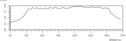
Figure 2 shows the potential distribution on the earth surface obtained by using the BEM approach; the graph of figure 3 represents the potential profile along a line (useful to obtain characteristical parameters such as step or touch voltage), and figure 4 shows a 3D view of the potential level on the earth surface when a fault condition occurs [6].
V(kV)
distance(m)
[image:2.595.316.550.172.257.2]Fig. 3. Barber´a grounding system: Potential profile along line in figure 2.
Fig. 4. Barber´a grounding system: 3D View of isopotential lines.
III. GROUNDINGANALYSIS INLAYEREDSOILMODELS
Next example corresponds to the grounding analysis of the Santiago II substation. In this example a comparison of results obtained by using a uniform soil model and a two layer soil one is presented. Table II summarizes the main characteristics of the earthing system and the soil models considered, as well as, the numerical model (582 linear boundary elements) and the results. Figure 5 shows the plan of the grounding grid.
TABLE II
SANTIAGOII GROUNDINGSYSTEM: CHARACTERISTICS, NUMERICAL MODEL& RESULTS
Data
Number of electrodes: 534 Number of ground rods: 24 Diameter of electrodes: 11.28 mm Diameter of ground rods: 15.00 mm Depth of the grid: 0.75 m Length of ground rods: 4 m Max. dimensions of grid: 230×195 m2
GPR: 10 kV
BEM Numerical Model Type of approach: Galerkin Type of 1D element: Linear
Number of elements: 582
Degrees of freedom: 386
One layer soil model Earth resistivity: 60Ωm
Total current: 6.73 kA
Equivalent resistance: 0.149Ω Two layer soil model Upper layer resistivity: 200Ωm Lower layer resistivity: 60Ωm Thickness upper layer: 1.2 m
Total current: 5.61 kA
Equivalent resistance: 0.178Ω
[image:2.595.358.517.453.679.2]1 Unit = 10 m
Fig. 5. Santiago II grounding grid plan.
0 50 100 150 200 250
[image:3.595.305.545.54.263.2]0 50 100 150 200
Fig. 6. Santiago II grounding system: Potential distribution (×10 kV) on the ground surface obtained with a homogeneous isotropic soil model.
in the lower one (the length of the ground rods is higher than the height of the upper layer). The complete discussion of this case can be found in [9].
As it is obvious, the results obtained by using a layer soil model are noticeably different from those obtained by using a uniform soil one. Since the safety grounding parameters computed from them significantly change, as a general rule it could be advisable to use efficient layer soil approaches to analyze grounding systems, in spite of the increase in the computational effort.
IV. TOTBEM: ANOPEN-SOURCECAD INTERFACE FOR
GROUNDINGANALYSIS
The numerical formulation based on the Boundary El-ement Method developed by the authors for uniform and layered soil models has been implemented in a freeware application for the in-house computer aided design and anal-ysis of grounding grids. The actual version of the software (TOTBEM) is available for testing purposes (and also use) at no cost and can be run on any basic personal computer (as of 2012) with no special requirements. The distribution
0 50 100 150 200 250
[image:3.595.49.288.270.478.2]0 50 100 150 200
Fig. 7. Santiago II grounding system: Potential distribution (×10 kV) on the ground surface obtained with a two-layer soil model.
Fig. 8. Santiago II grounding system: 3D visualizations of the potential distributions on the earth surface for the uniform (up), and the two-layer (down) soil models.
[image:3.595.312.547.313.652.2]Fig. 9. TOTBEM: Toolbox for preprocessing and input data.
Fig. 10. TOTBEM: Example of the input data for vertical rods.
software in the computer, but the application is still fully operational while the live DVD/USB is taking control. The pre- and post-processing engines of the application have been built on top of the open source SALOME platform toolkit [10].
The package TOTBEM includes all the preprocessing, computing and postprocessing stages necessary to perform a complete earthing analysis. The kernel of TOTBEM is the numerical formulation based on the BEM for uniform and stratified soil models including a high efficient technique to improve the rate of convergence of the involved series expansions in multilayer soil models [11].
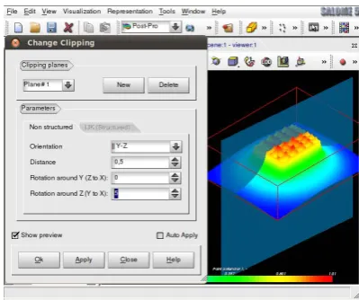
Figures 9 and 10 show examples of the TOTBEM pre-processing module for input data. Figure 11 shows the visualization of isopotential lines on the ground surface obtained from a grounding analysis and figure 12 is a 3D view of potential and isopotential lines of the same case.
V. TRANSFERRED EARTH POTENTIALS PROBLEM
In this section we briefly present a methodology for the analysis of a very important engineering problem in the grounding field: the problem of transferred earth potentials by grounded electrodes [12], that is, the phenomenon of the earth potential of one location appearing at another location with a contrasting earth potential. This transference occurs, for example, when a grounding grid is energized up to a certain voltage (tipically, the GPR) during a fault
Fig. 11. TOTBEM: Isopotential lines on the ground surface.
Fig. 12. TOTBEM: 3D view of potential and isopotential lines.
condition, and this voltage or a fraction of it appears out to a non-fault site by a buried or semiburied conductors (communication or signal circuits, neutral wires, metal pipes, rails, metallic fences, etc.). The danger that can imply these voltages to people, animals or the equipment is evident, and sometimes thety are produced in unexpected and non-protected areas [2]. The prevention of these transferred potentials has been traditionally carried out by combining a good engineering expertise, some crude calculations and even field measurements. In [13], the authors proposed a numerical methodology for the case of uniform soil models (generalized for stratified soil models in [14]) for the accurate determination of the transferred earth voltages by grounding grids by using computer methods.
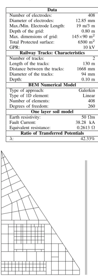
Table III summarizes main data of an application example of transferred earth potentials by a grounding grid due to the presence of railroad tracks in the vicinity of the substation site (often used to install high-power transformers or large equipment). Figure 13 shows the plan of the grounding grid of an electrical substation and the situation of the two tracks in the surroundings of the electrode.
[image:4.595.68.271.247.412.2] [image:4.595.325.525.248.415.2]TABLE III
BARBERA´-RAILWAYTRACKSGROUNDINGSYSTEM: CHARACTERISTICS, NUMERICAL MODEL& RESULTS
Data
Number of electrodes: 408 Diameter of electrodes: 12.85 mm Max./Min. Electrode Length: 19 m/3 m Depth of the grid: 0.80 m Max. dimensions of grid: 145×90 m2 Total Protected surface: 6500 m2
GPR: 10 kV
Railway Tracks: Characteristics
Number of tracks: 2
Length of the tracks: 130 m Distance between the tracks: 1668 mm Diameter of the tracks: 94 mm
Depth: 0.10 m
BEM Numerical Model Type of approach: Galerkin Type of 1D element: Linear
Number of elements: 408
Degrees of freedom: 260
One layer soil model
Earth resistivity: 50Ωm
Fault Current: 38.28 kA
Equivalent resistance: 0.2613Ω Ratio of Transferred Potentials
[image:5.595.335.519.50.328.2]λ: 42.33%
Fig. 13. Grounding grid plan and situation of the two railway tracks in the surroundings of the electrode.
VI. EARTHINGANALYSIS INHETEROGENEOUSSOILS: APPLICATION TOUNDERGROUNDSUBSTATIONS
In this section we present an example of grounding grids buried in soils which present some finite volumes with very different conductivities, which substantially differs from the layered ones. These type of models must be considered when a chemical treatment is applied to the soil in the surroundings of an earthing system to improve its operation, in soils with concrete foundations in the vicinity of the grounding grid, or in other practical situations such as swimming pools, soil de-pressions, lakes, grounding grids placed on rocky soil which conductors extent to a river (next to hydroelectric dams), or the grounding system of an underground electrical subtation. Although some particular cases could be approximated by using hemispherical soil models, obtaining accurate results
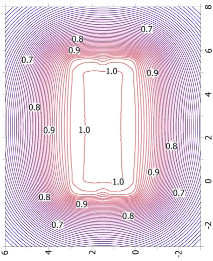
Fig. 14. Potential distribution (×10kV) on the earth surface during a fault condition considering the effect of the potential transferred by the tracks.
0.25 0.3 0.35 0.4 0.45 0.5 0.55 0.6 0.65 0.7 0.75 0.8 0.85 0.9 0.95
Fig. 15. TOTBEM Postprocessing module: 3D visualization of the potential distribution on the earth surface.
for soil models with finite volumes is only possible by using numerical methods [15].
Underground substations are very common in urban en-vironments where the space is limited. In this case, the substation is placed inside a monoblock concrete structure (which contains the transformers, switches and other elec-trical equipment) designed for installation underground. Fig. 16 shows schematically a typical monoblock concrete used to house the electrical substation (dimensions are l×w×
[image:5.595.94.262.77.549.2] [image:5.595.304.546.376.614.2]Fig. 16. Scheme of the monoblock concrete enclosure and the grounded electrode, formed by a ring buried 0.50 m from the earth surface and supplemented by four vertical rods with 4 m length.
quadrilateral ring placed to a distance of 0.8 m of the block, buried to a depth of 0.5 m and supplemented by vertical rods of 4 m length in each of its vertices. The diameter of the electrodes of the ring is 11.28 mm and the diameter of the vertical rods is 15.00 mm. The conductivity of the soil is 50 Ωm and the GPR is 10 kV [16].
The soil model of this problem can be considered as a particular case of an electrode embedded into the ground modeled as a uniform soil model which contains a finite volume (the concrete monoblock) with different conductivity (50 times lower than the soil). Fig. 17 shows the potential distribution on the earth surface in the vicinity of the substa-tion site and Fig. 18 shows a 3D view of the potential values on the earth surface. These results should be considered preliminary since the BEM numerical formulation is not yet fully implemented, but they show their capabilities to perform the grounding analysis of underground substations.
REFERENCES
[1] IEEE Std. 80,IEEE Guide for safety in AC substation grounding.New York, 2000.
[2] IEEE Std. 142,IEEE Recommended practice for grounding of indus-trial and commercial power systems.New York, 2007.
[3] J. G. Sverak, “Progress in step and touch voltage equations of ANSI/IEEE Std 80. Historical perspective”,IEEE Trans. Power Del., 13, (3), 762-767, July 1998.
[4] F. Navarrina, I. Colominas, and M. Casteleiro, “Why do computer methods for grounding produce anomalous results?”, IEEE Trans. Power Del.,18, (4), 1192-1202, Oct. 2003.
[5] D. L. Garrett and J. G. Pruitt, “Problems encountered with the average potential method of analyzing substation grounding systems”,IEEE Trans. Power App. Syst.,104, (12), 3586-3596, Dec. 1985.
[6] I. Colominas, F. Navarrina and M. Casteleiro,A boundary element formulation for the substation grounding design, Advances in Engi-neering Software,30, 693-700, (1999).
[7] I. Colominas, F. Navarrina, and M. Casteleiro, “A boundary element numerical approach for grounding grid computation”,Comput. Meth. Appl. Mech. Eng.,174, 73-90, 1999.
[8] I. Colominas, J. G´omez-Calvi˜no, F. Navarrina, and M. Casteleiro, “Computer analysis of earthing systems in horizontally and vertically layered soils”,Elect. Power Syst. Res.,59, 149-156, 2001.
[9] I. Colominas, F. Navarrina, and M. Casteleiro, “A numerical formu-lation for grounding analysis in stratified soils”,IEEE Trans. Power Del.,17, (2), 587-595, Apr. 2002.
[image:6.595.320.532.64.323.2]Fig. 17. Potential distribution on the earth surface (×10kV).
Fig. 18. 3D representation of the potential values on the earth surface.
[10] J. Par´ıs, I. Colominas, X. Nogueira, F. Navarrina, and M. Casteleiro, “Numerical simulation of multilayer grounding grids in a user-friendly open-source CAD interface”,Proceedings of the ICETCE–2012, IEEE Pub., New York, 2012
[11] I. Colominas, J. Par´ıs, F. Navarrina, and M. Casteleiro, “Improvement of the computer methods for grounding analysis in layered soils by using high-efficient convergence acceleration techniques”,Adv. Engrg. Soft.,44, 80-91, 2012
[12] Nichols N., Shipp D.D., “Designing to avoid hazardous transferred earth potentials”,IEEE Trans. Ind. Appl.,1A-18, 340–347, July 1982. [13] I. Colominas, F. Navarrina, and M. Casteleiro, “Analysis of transferred earth potentials in grounding systems: A BEM numerical approach”, IEEE Trans. Power Del.,20, (1), 339–345, Jan. 2005.
[14] I. Colominas, F. Navarrina, and M. Casteleiro, “Numerical Simulation of Transferred Potentials in Earthing Grids Considering Layered Soil Models”,IEEE Trans. Power Del.,22, (3), 1514–1522, July 2007. [15] J. Ma and F.P. Dawalibi, “Analysis of grounding systems in soils with
finite volumes of different resistivities”,IEEE Trans. Power Del.,17, 596-602, Apr. 2002.
[image:6.595.315.537.383.511.2]