Improving Accuracy in Word Class
Tagging through the Combination of
Machine Learning Systems
H a n s v a n H a l t e r e n * TOSCA/Language & Speech, University of Nijmegen
Walter Daelemans~
CNTS/Language Technology Group, University of Antwerp
Jakub Zavrel t
Textkernel BV,University of Antwerp
We examine how differences in language models, learned by different data-driven systems per- forming the same NLP task, can be exploited to yield a higher accuracy than the best individual system. We do this by means of experiments involving the task of morphosyntactic word class tagging, on the basis of three different tagged corpora. Four well-known tagger generators (hidden Markov model, memory-based, transformation rules, and maximum entropy) are trained on the same corpus data. After comparison, their outputs are combined using several voting strategies and second-stage classifiers. All combination taggers outperform their best component. The re- duction in error rate varies with the material in question, but can be as high as 24.3% with the LOB corpus.
1. Introduction
In all natural language processing (NLP) systems, we find one or more language models that are used to predict, classify, or interpret language-related observations. Because most real-world NLP tasks require something that approaches full language understanding in order to be perfect, but automatic systems only have access to limited (and often superficial) information, as well as limited resources for reasoning with that information, such language models tend to make errors when the system is tested on new material. The engineering task in NLP is to design systems that make as few errors as possible with as little effort as possible. Common ways to reduce the error rate are to devise better representations of the problem, to spend more time on encoding language knowledge (in the case of hand-crafted systems), or to find more training data (in the case of data-driven systems). However, given limited resources, these options are not always available.
Rather than devising a new representation for our task, in this paper, we combine different systems employing known representations. The observation that suggests this approach is that systems that are designed differently, either because they use a different formalism or because they contain different knowledge, will typically produce different errors. We hope to make use of this fact and reduce the number of errors with
Computational Linguistics Volume 27, Number 2
very little additional effort by exploiting the disagreement between different language models. Although the approach is applicable to any type of language model, we focus on the case of statistical disambiguators that are trained on annotated corpora. The examples of the task that are present in the corpus and its annotation are fed into a learning algorithm, which induces a model of the desired input-output mapping in the form of a classifier. We use a number of different learning algorithms simultaneously on the same training corpus. Each type of learning method brings its own "inductive bias" to the task and will produce a classifier with slightly different characteristics, so that different methods will tend to produce different errors.
We investigate two ways of exploiting these differences. First, we make use of the gang effect. Simply by using more than one classifier, and voting between their outputs, we expect to eliminate the quirks, and hence errors, that are due to the bias of one particular learner. However, there is also a w a y to make better use of the differences: we can create an arbiter effect. We can train a second-level classifier to select its output on the basis of the patterns of co-occurrence of the outputs of the various classifiers. In this way, we not only counter the bias of each component, but actually exploit it in the identification of the correct output. This method even admits the possibility of correcting collective errors. The hypothesis is that both types of approaches can yield a more accurate model from the same training data than the most accurate component of the combination, and that given enough training data the arbiter type of method will be able to outperform the gang type. 1
In the machine learning literature there has been much interest recently in the the- oretical aspects of classifier combination, both of the gang effect type and of the arbiter type (see Section 2). In general, it has been shown that, w h e n the errors are uncorre- lated to a sufficient degree, the resulting combined classifier will often perform better than any of the individual systems. In this paper we wish to take a more empirical approach and examine whether these methods result in substantial accuracy improve- ments in a situation typical for statistical NLP, namely, learning morphosyntactic word class tagging (also known as part-of-speech or POS tagging) from an annotated corpus of several hundred thousand words.
Morphosyntactic word class tagging entails the classification (tagging) of each token of a natural language text in terms of an element of a finite palette (tagset) of word class descriptors (tags). The reasons for this choice of task are several. First of all, tagging is a widely researched and well-understood task (see van Halteren [1999]). Second, current performance levels on this task still leave room for improvement: "state-of-the-art" performance for data-driven automatic word class taggers on the usual type of material (e.g., tagging English text with single tags from a low-detail tagset) is at 96-97% correctly tagged words, but accuracy levels for specific classes of ambiguous words are much lower. Finally, a number of rather different methods that automatically generate a fully functional tagging system from annotated text are available off-the-shelf. First experiments (van Halteren, Zavrel, and Daelemans 1998; Brill and Wu 1998) demonstrated the basic validity of the approach for tagging, with the error rate of the best combiner being 19.1% lower than that of the best individual tagger (van Halteren, Zavrel, and Daelemans 1998). However, these experiments were restricted to a single language, a single tagset and, more importantly, a limited amount of training data for the combiners. This led us to perform further, more extensive,
van Halteren, Zavrel, and Daelemans Combination of Machine Learning Systems
tagging experiments before moving on to other tasks. Since then the method has also been applied to other NLP tasks with good results (see Section 6).
In the remaining sections, we first introduce classifier combination on the basis of previous work in the machine learning literature and present the combination meth- ods we use in our experiments (Section 2). Then we explain our experimental setup (Section 3), also describing the corpora (3.1) and tagger generators (3.2) used in the experiments. In Section 4, we go on to report the overall results of the experiments, starting with a comparison between the component taggers (and hence between the underlying tagger generators) and continuing with a comparison of the combination methods. The results are examined in more detail in Section 5, where we discuss such aspects as accuracy on specific words or tags, the influence of inconsistent training data, training set size, the contribution of individual component taggers, and tagset granularity. In Section 6, we discuss the results in the light of related work, after which we conclude (Section 7) with a summary of the most important observations and interesting directions for future research.
2. Combination Methods
In recent years there has been an explosion of research in machine learning on finding ways to improve the accuracy of supervised classifier learning methods. An important finding is that a set of classifiers whose individual decisions are combined in some w a y (an ensemble) can be more accurate than any of its component classifiers if the errors of the individual classifiers are sufficiently uncorrelated (see Dietterich [1997], Chan, Stolfo, and Wolpert [1999] for overviews). There are several ways in which an ensemble can be created, both in the selection of the individual classifiers and in the w a y they are combined.
One w a y to create multiple classifiers is to use subsamples of the training exam- ples. In bagging, the training set for each individual classifier is created b y randomly drawing training examples with replacement from the initial training set (Breiman 1996a). In boosting, the errors made by a classifier learned from a training set are used to construct a new training set in which the misclassified examples get more weight. By sequentially performing this operation, an ensemble is constructed (e.g., ADABOOST, [Freund and Schapire 1996]). This class of methods is also called arcing (for adaptive resampling and combining). In general, boosting obtains better results than bagging, except when the data is noisy (Dietterich 1997). Another w a y to cre- ate multiple classifiers is to train classifiers on different sources of information about the task b y giving them access to different subsets of the available input features (Cherkauer 1996). Still other ways are to represent the output classes as bit strings where each bit is predicted by a different component classifier (error correcting output coding [Dietterich and Bakiri 1995]) or to develop learning-method-specific methods for ensuring (random) variation in the w a y the different classifiers of an ensemble are constructed (Dietterich 1997).
In this paper we take a multistrategy approach, in which an ensemble is con- structed by classifiers resulting from training different learning methods on the same data (see also Alpaydin [1998]).
Computational Linguistics Volume 27, Number 2
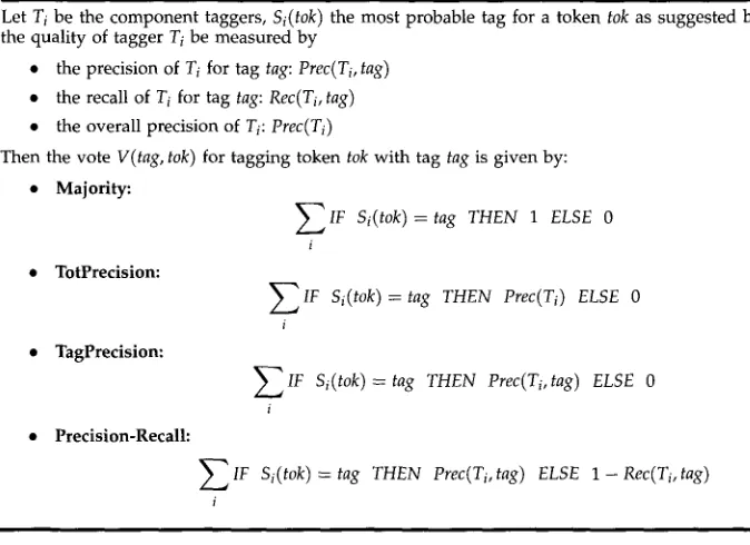
Let Ti be the component taggers, Si(tok) the most probable tag for a token tok as suggested by Ti, and let the quality of tagger T i be measured by
• the precision of Ti for tag tag: Prec(Ti, tag) • the recall of T i for tag tag: Rec(Ti, tag) • the overall precision of Ti: Prec(Ti)
Then the vote V(tag, tok) for tagging token tok with tag tag is given by:
• Majority:
• TotPrecision:
• TagPrecision:
• Precision-Recall:
~ _ I F Si(tok)= tag THEN 1 ELSE 0 i
~ _ I F Si(tok)= tag THEN Prec(Ti) ELSE 0 i
~__IF Si(tok ) = tag THEN Prec(Ti, tag) ELSE 0 i
[image:4.468.50.387.55.300.2]~_.IF Si(tok ) =tag THEN Prec(Ti, tag) ELSE 1-Rec(Ti, tag) i
Figure 1
Simple algorithms for voting between component taggers.
most interesting a p p r o a c h to c o m b i n a t i o n is stacking in w h i c h a classifier is trained to predict the correct o u t p u t class w h e n g i v e n as i n p u t the o u t p u t s of the ensemble classifiers, a n d possibly additional i n f o r m a t i o n (Wolpert 1992; Breiman 1996b; Ting a n d Witten 1997a, 1997b). Stacking can lead to an arbiter effect. In this p a p e r w e c o m p a r e v o t i n g a n d stacking a p p r o a c h e s o n the tagging problem.
In the r e m a i n d e r of this section, w e describe the c o m b i n a t i o n m e t h o d s w e use in o u r experiments. We start w i t h variations b a s e d on w e i g h t e d voting. T h e n w e go o n to several types of stacked classifiers, w h i c h m o d e l the d i s a g r e e m e n t situations o b s e r v e d in the training data in m o r e detail. The i n p u t to the second-stage classifier can be limited to the first-level o u t p u t s or can contain additional i n f o r m a t i o n f r o m the original i n p u t pattern. We will consider a n u m b e r of different second-level learners. A p a r t f r o m using three w e l l - k n o w n m a c h i n e learning m e t h o d s , m e m o r y - b a s e d learn- ing, m a x i m u m entropy, a n d decision trees, w e also i n t r o d u c e a n e w m e t h o d , b a s e d o n g r o u p e d voting.
2.1 Simple Voting
The most s t r a i g h t f o r w a r d m e t h o d to c o m b i n e the results of multiple taggers is to d o an n - w a y vote. Each tagger is a l l o w e d to vote for the tag of its choice, a n d the tag w i t h the highest n u m b e r of votes is selected. 2 The q u e s t i o n is h o w large a vote w e allow each tagger (Figure 1). The most democratic o p t i o n is to give each tagger one vote (Majority). This does not require a n y t u n i n g of the v o t i n g m e c h a n i s m on training data. H o w e v e r , the c o m p o n e n t taggers can be distinguished b y several figures of merit, a n d it a p p e a r s m o r e useful to give m o r e w e i g h t to taggers that h a v e p r o v e d their quality. For this p u r p o s e w e use p r e c i s i o n a n d recall, t w o w e l l - k n o w n measures, w h i c h
van Halteren, Zavrel, and Daelemans Combination of Machine Learning Systems
can be applied to the evaluation of tagger output as well. For any tag X, precision measures which percentage of the tokens tagged X by the tagger are also tagged X in the benchmark. Recall measures which percentage of the tokens tagged X in the benchmark are also tagged X by the tagger. When abstracting away from individual tags, precision and recall are equal (at least if the tagger produces exactly one tag per token) and measure how many tokens are tagged correctly; in this case we also use the more generic term accuracy. We will call the voting method where each tagger is weighted by its general quality TotPrecision, i.e., each tagger votes its overall precision. To allow for more detailed interactions, each tagger is weighted by the quality in relation to the current situation, i.e., each tagger votes its precision on the tag it suggests
(TagPrecision).
This way, taggers that are accurate for a particular type of ambiguity can act as specialized experts. The information about each tagger's quality is derived from a cross-validation of its results on the combiner training set. The precise setup for deriving the training data is described in more detail below, in Section 3.We have access to even more information on how well the taggers perform. We not only know whether we should believe what they propose (precision) but know as well how often they fail to recognize the correct tag (1 - recall). This information can be used by forcing each tagger to add to the vote for tags suggested by the opposition too, by an amount equal to 1 minus the recall on the opposing tag (Precision-Recall). As an example, suppose that the MXPOST tagger suggests DT and the HMM tagger TnT suggests CS (two possible tags in the LOB tagset for the token that). If MXPOST has a precision on DT of 0.9658 and a recall on CS of 0.8927, and TnT has a precision on CS of 0.9044 and a recall on DT of 0.9767, then DT receives a 0.9658 + 0.0233 = 0.9991 vote and CS a 0.9044 + 0.1073 = 1.0117 vote.
Note that simple voting combiners can never return a tag that was not suggested by a (weighted) majority of the component taggers. As a result, they are restricted to the combination of taggers that all use the same tagset. This is not the case for all the following (arbiter type) combination methods, a fact which we have recently exploited in bootstrapping a word class tagger for a new corpus from existing taggers with completely different tagsets (Zavrel and Daelemans 2000).
2.2 Stacked Probabilistic Voting
One of the best methods for tagger combination in (van Halteren, Zavrel, and Daele- mans 1998) is the TagPair method. It looks at all situations where one tagger suggests tag 1 and the other tag 2 and estimates the probability that in this situation the tag should actually be tag x. Although it is presented as a variant of voting in that paper, it is in fact also a stacked classifier, because it does not necessarily select one of the tags suggested by the component taggers. Taking the same example as in the voting section above, if tagger MXPOST suggests DT and tagger TnT suggests CS, we find that the probabilities for the appropriate tag are:
CS CS22 DT QL WPR
subordinating conjunction 0.4623
second half of a two-token subordinating conjunction, e.g., so that 0.0171
determiner 0.4966
quantifier 0.0103
wh-pronoun 0.0137
Computational Linguistics Volume 27, Number 2
Let Ti be the component taggers and Si(tok) the most probable tag for a token tok as suggested by Ti. Then the vote V(tag, tok) for tagging token tok with tag tag is given by:
V(tag, tok) = ~_~ Vi,j(tag , tok) i,jliKj
where Vial(tag, tok) is given by
IF frequency(Si(tokx) = Si(tok), Sj(tokx) = Sj(tok) ) > 0
THEN Vial(tag, tok) = P(tag l Si(tok~) = Si(tok), Sj(tokx) = Sj(tok) )
Vi,j(tag, tok) = ~P(tag ] Si(tokx) = Si(tok) ) + ~P(tag I Sj(tokx) = Sj(tok) ) ELSE
Figure 2
The TagPair algorithm for voting between component taggers. If the case to be classified corresponds to the feature-value pair set
Fcase = {0Cl = V l } . . . {fn = V n } }
then estimate the probability of each class Cx for Fcase as a weighted sum over all possible subsets Fsu b of Fcase:
~(Cx)
~_, Wr~.bP(CK
I Esub) Fsub C Fcasewith the weight WG, b for an Fsub containing n elements equal to n---L-r' where Wnor m i Wnorm is a normalizing constant so that ~ c x P(Cx) = 1.
Figure 3
The Weighted Probability Distribution Voting classification algorithm, as used in the combination experiments.
a n d P ( t a g x I tag2). N o t e that w i t h this m e t h o d (and all of the following), a t a g s u g g e s t e d b y a m i n o r i t y (or e v e n none) of the t a g g e r s a c t u a l l y h a s a chance to win, a l t h o u g h in practice the chance to b e a t a m a j o r i t y is still v e r y slight.
Seeing the success of TagPair in the earlier e x p e r i m e n t s , w e d e c i d e d to t r y to generalize this s t a c k e d probabilistic v o t i n g a p p r o a c h to c o m b i n a t i o n s larger t h a n pairs. A m o n g other things, this w o u l d let us include w o r d a n d context features h e r e as well. T h e m e t h o d that w a s e v e n t u a l l y d e v e l o p e d w e h a v e called
Weighted Probability
Distribution Voting
(henceforth WPDV).A W P D V classification m o d e l is n o t limited to p a i r s of features (such as the pairs of t a g g e r o u t p u t s for TagPair), b u t can u s e the p r o b a b i l i t y distributions for all feature c o m b i n a t i o n s o b s e r v e d in the training d a t a (Figure 3). D u r i n g v o t i n g , w e d o n o t u s e a fallback s t r a t e g y (as TagPair does) b u t u s e w e i g h t s to p r e v e n t the l o w e r - o r d e r c o m b i - n a t i o n s f r o m excessively influencing the final results w h e n a h i g h e r - o r d e r c o m b i n a t i o n (i.e., m o r e exact i n f o r m a t i o n ) is present. The original s y s t e m , as u s e d for this p a p e r , w e i g h t s a c o m b i n a t i o n of o r d e r n w i t h a factor n!, a n u m b e r b a s e d o n the o b s e r v a t i o n that a c o m b i n a t i o n of o r d e r m contains m c o m b i n a t i o n s of o r d e r (m - 1) t h a t h a v e to b e c o m p e t e d with. Its o n l y p a r a m e t e r is a t h r e s h o l d for the n u m b e r of times a c o m b i - n a t i o n m u s t b e o b s e r v e d in the training d a t a in o r d e r to be used, w h i c h h e l p s p r e v e n t a c o m b i n a t o r i a l e x p l o s i o n w h e n there are too m a n y a t o m i c features. 3
van Halteren, Zavrel, and Daelemans Combination of Machine Learning Systems
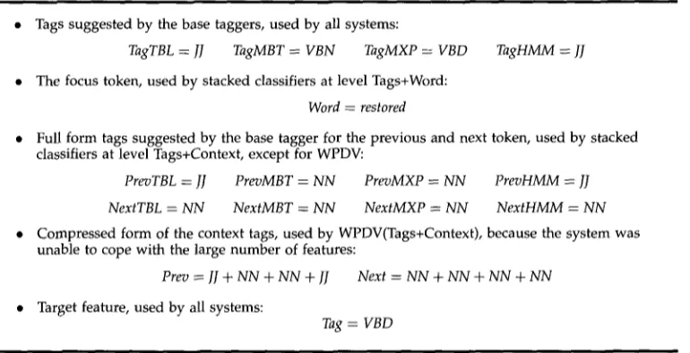
• Tags suggested by the base taggers, used by all systems:
TagTBL = JJ T a g M B T = V B N T a g M X P = V B D T a g H M M = JJ
• The focus token, used by stacked classifiers at level Tags+Word: W o r d = restored
• Full form tags suggested by the base tagger for the previous and next token, used by stacked classifiers at level Tags+Context, except for WPDV:
P r e v T B L = JJ P r e v M B T = N N P r e v M X P = N N P r e v H M M = J]
N e x t T B L = N N N e x t M B T = N N N e x t M X P = N N N e x t H M M = N N • Compressed form of the context tags, used by WPDV(Tags+Context), because the system was
unable to cope with the large number of features:
P r e v ~- JJ + N N + N N + JJ N e x t = N N + N N + N N + N N
• Target feature, used by all systems:
[image:7.468.39.424.55.252.2]Tag = V B D
Figure 4
Features used by the combination systems. Examples are taken from the LOB material.
In contrast to voting, stacking classifiers allows the c o m b i n a t i o n of the o u t p u t s of c o m p o n e n t systems w i t h additional i n f o r m a t i o n a b o u t the decision's context. We in- vestigated several versions of this approach. In the basic version (Tags), each training case for the second-level learner consists of the tags suggested b y the c o m p o n e n t tag- gers a n d the correct tag (Figure 4). In the m o r e a d v a n c e d versions, w e a d d i n f o r m a t i o n a b o u t the w o r d in question (Tags+Word) a n d the tags suggested b y all taggers for the p r e v i o u s and the next position (Tags+Context). These types of e x t e n d e d second-level features can be exploited b y WPDV, as well as b y a w i d e selection of other m a c h i n e learning algorithms.
2.3 Memory-based Combination
O u r first choice f r o m these other algorithms is a m e m o r y - b a s e d second-level learner, i m p l e m e n t e d in TiMBL (Daelemans et al. 1999), a p a c k a g e d e v e l o p e d at Tilburg Uni- versity and A n t w e r p University. 4
M e m o r y - b a s e d learning is a learning m e t h o d that is b a s e d on storing all examples of a task in m e m o r y a n d then classifying n e w examples b y similarity-based reasoning f r o m these stored examples. Each e x a m p l e is r e p r e s e n t e d b y a fixed-length vector of feature values, called a case. If the case to be classified has b e e n o b s e r v e d before, that is, if it is f o u n d a m o n g the stored cases (in the case base), the m o s t frequent c o r r e s p o n d i n g o u t p u t is used. If the case is not f o u n d in the case base, k nearest neighbors are d e t e r m i n e d with some similarity metric, a n d the o u t p u t is based o n the o b s e r v e d o u t p u t s for those neighbors. Both the value of k a n d the similarity metric used can be selected b y p a r a m e t e r s of the system. For the Tags version, the similarity metric u s e d is O v e r l a p (a c o u n t of the n u m b e r of m a t c h i n g feature values b e t w e e n a test a n d a training item) and k is kept at 1. For the other t w o versions (Tags+Word a n d Tags+Context), a v a l u e of k = 3 is used, a n d each o v e r l a p p i n g feature is w e i g h t e d b y its Information Gain (Daelemans, Van d e n Bosch, a n d Weijters 1997). The I n f o r m a t i o n
Computational Linguistics Volume 27, Number 2
Gain of a feature is defined as the difference between the entropy of the a priori class distribution and the conditional entropy of the classes given the value of the feature. ~ 2.4 Maximum Entropy Combination
The second machine learning method, m a x i m u m entropy modeling, i m p l e m e n t e d in the Maccent system (Dehaspe 1997), does the classification task b y selecting the most probable class given a m a x i m u m entropy model. 6 This type of model represents ex- amples of the task (Cases) as sets of binary indicator features, for the task at h a n d conjunctions of a particular tag a n d a particular set of feature values. The model has the form of an exponential model:
1 e Y~i ~i~(ca~,~g) pA(tag l Case) -- Za(Case)
where i indexes all the b i n a r y features, fi is a binary indicator function for feature i, ZA is a normalizing constant, a n d
)~i
is a w e i g h t for feature i. The m o d e l is trained b y iteratively a d d i n g binary features w i t h the largest gain in the probability of the train- ing data, a n d estimating the weights using a numerical optimization m e t h o d called i m p r o v e d iterafive scaling. The m o d e l is constrained b y the observed distribution of the features in the training data a n d has the p r o p e r t y of having the m a x i m u m en- tropy of all models that fit the constraints, i.e., all distributions that are not directly constrained b y the data are left as u n i f o r m as possible. 7The m a x i m u m entropy combiner takes the same information as the m e m o r y - b a s e d learner as input, b u t internally translates all m u l t i v a l u e d features to binary indicator functions. The i m p r o v e d iterative scaling algorithm is then applied, w i t h a m a x i m u m of one h u n d r e d iterations. This algorithm is the same as the one used in the M X P O S T tagger described in Section 3.2.3, b u t w i t h o u t the b e a m search used in the tagging application.
2.5 Decision Tree Combination
The third machine learning m e t h o d we u s e d is c5.0 (Quinlan 1993), an example of t o p - d o w n induction of decision trees. 8 A decision tree is constructed b y recursively partitioning the training set, selecting, at each step, the feature that most reduces the uncertainty about the class in each partition, a n d using it as a split, c5.0 uses Gain Ratio as an estimate of the utility of splitting on a feature. Gain Ratio corresponds to the Information Gain measure of a feature, as described above, except that the measure is normalized for the n u m b e r of values of the feature, b y dividing b y the entropy of the feature's values. After the decision tree is constructed, it is p r u n e d to avoid overfitting, using a m e t h o d described in detail in Quinlan (1993). A classification for a test case is m a d e b y traversing the tree until either a leaf n o d e is f o u n d or all further branches do not m a t c h the test case, a n d returning the most frequent class at the last node. The case representation uses exactly the same features as the m e m o r y - b a s e d learner. 3. Experimental Setup
In order to test the potential of system combination, w e obviously need systems to combine, i.e., a n u m b e r of different taggers. As we are primarily interested in the
5 This is also sometimes referred to as mutual information in the computational linguistics literature. 6 Maccent is available from http://www.cs.kuleuven.ac.be/~ldh.
7 For a more detailed discussion, see Berger, Della Pietra, and Della Pietra (1996) and Ratnaparkhi (1996). 8 c5.0 is commercially available from http://www.rulequest.com/. Its predecessor, c4.5, can be
van Halteren, Zavrel, and Daelemans Combination of Machine Learning Systems
c o m b i n a t i o n of classifiers trained on the same data sets, w e are in fact looking for data sets (in this case, t a g g e d corpora) a n d systems that can automatically gener- ate a tagger o n the basis of those data sets. For the current experiments, w e h a v e selected three tagged c o r p o r a a n d four tagger generators. Before giving a detailed description of each of these, w e first describe h o w the ingredients are u s e d in the experiments.
Each c o r p u s is u s e d in the same w a y to test tagger a n d c o m b i n e r p e r f o r m a n c e . First of all, it is split into a 90% training set a n d a 10% test set. We can evaluate the base taggers b y using the w h o l e training set to train the tagger generators a n d the test set to test the resulting tagger. For the combiners, a m o r e c o m p l e x strategy m u s t be followed, since c o m b i n e r training m u s t be d o n e on material u n s e e n b y the base taggers involved. Rather than setting apart a fixed c o m b i n e r training set, w e use a ninefold training strategy? The 90% trai1~ing set is split into nine equal parts. Each p a r t is t a g g e d with c o m p o n e n t taggers that h a v e b e e n trained o n the other eight parts. All results are then concatenated for use in c o m b i n e r training, so that, in contrast to o u r earlier work, all of the training set is effectively available for the training of the combiner. Finally, the resulting combiners are tested on the test set. Since the test set is identical for all m e t h o d s , w e can c o m p u t e the statistical significance of the results using M c N e m a r ' s chi-squared test (Dietterich 1998).
As w e will see, the increase in c o m b i n e r training set size (90% of the c o r p u s versus the fixed 10% tune set in the earlier experiments) i n d e e d results in better p e r f o r m a n c e . O n the other h a n d , the increased a m o u n t of data also increases time a n d space require- m e n t s for some systems to such a degree that w e h a d to exclude t h e m f r o m (some parts of) the experiments.
The data in the training set is the o n l y i n f o r m a t i o n u s e d in tagger a n d c o m b i n e r construction: all c o m p o n e n t s of all taggers a n d combiners (lexicon, context statistics, etc.) are entirely data driven, and no m a n u a l adjustments are made. If a n y tagger or c o m b i n e r construction m e t h o d is p a r a m e t r i z e d , w e use default settings w h e r e avail- able. If there is no default, w e choose intuitively a p p r o p r i a t e values w i t h o u t prelimi- n a r y testing. In these cases, w e r e p o r t such p a r a m e t e r settings in the i n t r o d u c t i o n to the system.
3.1 Data
In the current e x p e r i m e n t s w e m a k e use of three corpora. The first is the LOB c o r p u s (Johansson 1986), w h i c h w e used in the earlier e x p e r i m e n t s as well (van Halteren, Zavrel, and Daelemans 1998) and w h i c h has p r o v e d to be a g o o d testing g r o u n d . We t h e n switch to Wall Street Journal material (WSJ), t a g g e d with the P e n n Treebank II tagset (Marcus, Santorini, a n d Marcinkiewicz 1993). Like LOB, it consists of approx- imately 1M words, b u t unlike LOB, it is A m e r i c a n English. F u r t h e r m o r e , it is of a different structure (only n e w s p a p e r text) a n d tagged with a rather different tagset. The e x p e r i m e n t s w i t h WSJ will also let us c o m p a r e o u r results with those r e p o r t e d b y Brill a n d Wu (1998), w h i c h s h o w a m u c h less p r o n o u n c e d accuracy increase than ours with LOB. The final c o r p u s is the slightly smaller (750K words) E i n d h o v e n c o r p u s (Uit d e n Boogaart 1975) tagged w i t h the Wotan tagset (Berghmans 1994). This will let us examine the tagging of a language other than English (namely, Dutch). F u r t h e r m o r e , the Wotan tagset is a v e r y detailed one, so that the error rate of the i n d i v i d u a l taggers
Computational Linguistics Volume 27, N u m b e r 2
t e n d s to b e higher. M o r e o v e r , w e c a n m o r e easily u s e p r o j e c t i o n s of the t a g s e t a n d t h u s s t u d y the effects of levels of g r a n u l a r i t y .
3.1.1 L O B . T h e first d a t a set w e u s e for o u r e x p e r i m e n t s consists of t h e t a g g e d L a n c a s t e r - O s l o / B e r g e n c o r p u s (LOB [ J o h a n s s o n 1986]). T h e c o r p u s c o m p r i s e s a b o u t o n e m i l l i o n w o r d s of British E n g l i s h text, d i v i d e d o v e r 500 s a m p l e s of 2,000 w o r d s f r o m 15 text t y p e s .
T h e t a g g i n g of the L O B c o r p u s , w h i c h w a s m a n u a l l y c h e c k e d a n d c o r r e c t e d , is g e n e r a l l y a c c e p t e d to b e q u i t e accurate. H e r e w e u s e a slight a d a p t a t i o n of t h e tagset. T h e c h a n g e s are m a i n l y c o s m e t i c , e.g., n o n a l p h a b e t i c c h a r a c t e r s s u c h as " $ " in t a g n a m e s h a v e b e e n r e p l a c e d . H o w e v e r , t h e r e h a s also b e e n s o m e r e t o k e n i z a t i o n : g e n i t i v e m a r k e r s h a v e b e e n split off a n d the n e g a t i v e m a r k e r n't h a s b e e n r e a t t a c h e d .
A n e x a m p l e s e n t e n c e t a g g e d w i t h t h e r e s u l t i n g t a g s e t is:
The ATI singular or plural article Lord NPT singular titular noun Major NPT singular titular noun extended VBD past tense of verb
an AT singular article
invitation NN singular common noun
to IN preposition
all ABN pre-quantifier
the ATI singular or plural article parliamentary JJ adjective
candidates NNS plural common noun SPER period
T h e t a g s e t consists of 170 d i f f e r e n t t a g s ( i n c l u d i n g ditto tags), a n d h a s a n a v e r a g e a m b i g u i t y of 2.82 t a g s p e r w o r d f o r m o v e r t h e c o r p u s . 1° A n i m p r e s s i o n of the difficulty of t h e t a g g i n g t a s k c a n b e g a i n e d f r o m t h e t w o b a s e l i n e m e a s u r e m e n t s in Table 2 (in Section 4.1 b e l o w ) , r e p r e s e n t i n g a c o m p l e t e l y r a n d o m c h o i c e f r o m t h e p o t e n t i a l t a g s for e a c h t o k e n ( R a n d o m ) a n d selection of t h e lexically m o s t likely t a g ( L e x P r o b ) J 1
T h e t r a i n i n g / t e s t s e p a r a t i o n of the c o r p u s is d o n e at u t t e r a n c e b o u n d a r i e s (each 1st to 9 t h u t t e r a n c e is t r a i n i n g a n d e a c h 10th is test) a n d l e a d s to a 1,046K t o k e n t r a i n i n g set a n d a 115K t o k e n test set. A r o u n d 2.14% of t h e test set are t o k e n s u n s e e n in t h e t r a i n i n g set a n d a f u r t h e r 0.37% are k n o w n t o k e n s b u t w i t h u n s e e n tags. 12
3.1.2 WSJ. T h e s e c o n d d a t a set consists of 1M w o r d s of Wall Street Journal m a t e r i a l . It differs f r o m L O B in t h a t it is A m e r i c a n E n g l i s h a n d , m o r e i m p o r t a n t l y , in t h a t it is c o m p l e t e l y m a d e u p of n e w s p a p e r text. T h e m a t e r i a l is t a g g e d w i t h t h e P e n n T r e e b a n k t a g s e t (Marcus, Santorini, a n d M a r c i n k i e w i c z 1993), w h i c h is m u c h s m a l l e r t h a n t h e L O B one. It consists of o n l y 48 tags. 13 T h e r e is n o a t t e m p t to a n n o t a t e c o m p o u n d w o r d s , so t h e r e are n o ditto tags.
10 Ditto tags are used for the components of multitoken units, e.g. if as well as is taken to be a coordinating conjunction, it is tagged "as_CC-1 well_CC-2 as_CC-3", using three related but different ditto tags. 11 These numbers are calculated on the basis of a lexicon derived from the whole corpus. An actual
tagger will have to deal with unknown words in the test set, which will tend to increase the ambiguity and decrease Random and LexProb. Note that all actual taggers and combiners in this paper do have to cope with unknown words as their lexicons are based purely on their training sets.
12 Because of the way in which the tagger generators treat their input, we do count tokens as different even though they are the same underlying token, but differ in capitalization of one or more characters. 13 In the material we have available, quotes are represented slightly differently, so that there are only 45
van Halteren, Zavrel, and Daelemans Combination of Machine Learning Systems
An e x a m p l e sentence is:
By IN preposition/subordinating conjunction
10 CD cardinal number
a.m. RB adverb
Tokyo NNP singular proper noun
time NN singular common noun
comma
the E)T determiner
index NN singular common noun
was VBD past tense verb
up RB adverb
435.11 CD cardinal number
points NNS plural common noun
comma t o ,,to,,
34903.80 CD cardinal number
as IN preposition/subordinating conjunction
investors NNS plural common noun hailed VBD past tense verb
New NNP singular proper noun
York NNP singular proper noun
's POS possessive ending
overnight JJ adjective
rally NN singular common noun
sentence-final punctuation
Mostly because of the less detailed tagset, the average a m b i g u i t y of the tags is l o w e r than LOB's, at 2.34 tags per t o k e n in the corpus. This m e a n s that the tagging task s h o u l d be an easier one than that for LOB. This is s u p p o r t e d b y the values for R a n d o m and LexProb in Table 2. On the other h a n d , the less detailed tagset also m e a n s that the taggers h a v e less detailed i n f o r m a t i o n to base their decisions on. A n o t h e r factor that influences the quality of automatic tagging is the consistency of the tagging o v e r the corpus. The WSJ material has n o t b e e n checked as extensively as the LOB c o r p u s a n d is e x p e c t e d to h a v e a m u c h l o w e r consistency level (see Section 5.3 b e l o w for a closer examination).
The t r a i n i n g / t e s t separation of the c o r p u s is again d o n e at utterance b o u n d a r i e s a n d leads to a 1,160K t o k e n training set a n d a 129K t o k e n test set. A r o u n d 1.86% of the test set are u n s e e n tokens a n d a f u r t h e r 0.44% are k n o w n tokens w i t h p r e v i o u s l y u n s e e n tags.
3.1.3 E i n d h o v e n . The final two data sets are b o t h b a s e d on the E i n d h o v e n c o r p u s (Uit d e n Boogaart 1975). This is slightly smaller than LOB a n d WSJ. The written part, w h i c h w e use in o u r experiments, consists of a b o u t 750K w o r d s , in samples ranging from 53 to 451 words. In variety, it lies b e t w e e n LOB a n d WSJ, containing 150K w o r d s each of samples from D u t c h n e w s p a p e r s (subcorpus CDB), weeklies (OBL), m a g a z i n e s (GBL), p o p u l a r scientific writings (PWE), a n d novels (RNO).
Computational Linguistics Volume 27, N u m b e r 2
w e also d e s i g n e d a s i m p l i f i c a t i o n of the tagset, d u b b e d W o t a n L i t e , w h i c h n o l o n g e r c o n t a i n s the m o s t p r o b l e m a t i c distinctions. W o t a n L i t e h a s 129 t a g s ( w i t h a c o m p l e m e n t of ditto t a g s l e a d i n g to a total of 173) a n d a n a v e r a g e a m b i g u i t y of 3.46 t a g s p e r t o k e n . A n e x a m p l e of W o t a n t a g g i n g is g i v e n b e l o w ( o n l y u n d e r l i n e d p a r t s r e m a i n in WotanLite): 14
Mr. (Master, t i t l e ) N(eigen,ev, neut):l/2
Rijpstra N(eigen,ev, neut):2/2
heeft (has) V(hulp,ott,3,ev)
de (the) Art(bep,zijd-of-mv, neut)
Commissarispost N(soort,ev, neut)
(post of Commissioner)
in (in) Prep(voor)
Friesland N(eigen,ev, neut)
geambieerd (aspired to) V(trans,verl-dw, onverv)
en (and) Conj(neven)
hij (he) Pron(per,3,ev, nom)
moet (should) V(hulp,ott,3,ev)
dus (therefore) Adv(gew, aanw)
alle ( a l l ) Pron(onbep,neut,attr)
kans (opportunity) N_~(soort,ev, neut) hebben (have) V__((trans,inf)
er (there) Adv(pron,er)
het (the) Art(bep,onzijd,neut)
beste (best) Adj (zelfst,over tr,verv-neut)
van (of) Adv(deel-adv)
te (to) Prep(voor-inf)
maken (make) V(trans,inf) Punc(punt)
first part of singular neutral case proper noun second part of singular neutral case proper
noun
3rd person singular present tense auxiliary verb neutral case non-neuter or plural definite article singular neutral case common noun
adposition used as preposition singular neutral case proper noun
base form of past participle of transitive verb coordinating conjunction
3rd person singular nominative personal pronoun
3rd person singular present tense auxiliary verb demonstrative non-pronominal adverb
attributively used neutral case indefinite pronoun
singular neutral case common noun infinitive of transitive verb pronominal adverb "er"
neutral case neuter definite article nominally used inflected superlative
form of adjective particle adverb infinitival "te"
infinitive of transitive verb period
T h e a n n o t a t i o n of t h e c o r p u s w a s r e a l i z e d b y a s e m i a u t o m a t i c u p g r a d e of the t a g g i n g i n h e r i t e d f r o m a n earlier project. T h e r e s u l t i n g c o n s i s t e n c y h a s n e v e r b e e n e x h a u s t i v e l y m e a s u r e d for e i t h e r t h e W o t a n or t h e o r i g i n a l t a g g i n g .
T h e t r a i n i n g / t e s t s e p a r a t i o n of the c o r p u s is d o n e at s a m p l e b o u n d a r i e s (each 1st to 9 t h s a m p l e is t r a i n i n g a n d e a c h 10th is test). This is a m u c h stricter s e p a r a t i o n t h a n a p p l i e d for L O B a n d WSJ, as f o r t h o s e t w o c o r p o r a o u r test u t t e r a n c e s are r e l a t e d to t h e t r a i n i n g o n e s b y b e i n g in t h e s a m e s a m p l e s . P a r t l y as a r e s u l t of this, b u t also v e r y m u c h b e c a u s e of w o r d c o m p o u n d i n g in D u t c h , w e see a m u c h h i g h e r p e r c e n t a g e of n e w t o k e n s - - 6 . 2 4 % t o k e n s u n s e e n in the t r a i n i n g set. A f u r t h e r 1.45% k n o w n t o k e n s h a v e n e w t a g s for W o t a n , a n d 0.45% for W o t a n L i t e . T h e t r a i n i n g set consists of 640K t o k e n s a n d t h e test set of 72K t o k e n s .
3.2 Tagger Generators
T h e s e c o n d i n g r e d i e n t f o r o u r e x p e r i m e n t s is a set of f o u r t a g g e r g e n e r a t o r s y s t e m s , selected o n t h e basis of v a r i e t y a n d availability, is E a c h of t h e s y s t e m s r e p r e s e n t s a
14 The example sentence could be rendered in English as Master Rijpstra has aspired to the post of Commissioner in Friesland and he should therefore be given every opportunity to make the most of it.
van Halteren, Zavrel, and Daelemans Combination of Machine Learning Systems
Table 1
The features available to the four taggers in our study. Except for MXPOST, all systems use different models (and hence features) for known (k) and unknown (u) words. However, Brill's transformation-based learning system (TBL) applies its two models in sequence when faced with unknown words, thus giving the unknown-word tagger access to the features used by the known-word model as well. The first five columns in the table show features of the focus word: capitalization (C), hyphen (H), or digit (D) present, and number of suffix (S) or prefix (P) letters of the word. Brill's TBL system (for unknown words) also takes into account whether the addition or deletion of a suffix results in a known lexicon entry (indicated by an L). The next three columns represent access to the actual word (W) and any range of words to the left
(Wleft)
o r right (Wright). The last three columns show access to tag information for theword itself (T) and any range of words left (Tleft) or right (Tright). Note that the expressive power of a method is not purely determined by the features it has access to, but also by its algorithm, and what combinations of the available features this allows it to consider.
Features
System C D N S P W Wtedt Wright T Tteft
Zright
TBL (k) x 1-2 1-2 x 1-3 1-3
TBL (u) x x x 4,L 4,L 1-2 1-2 1-3 1-3
MBT (k) x x 1-2 1-2
MBT (u) x x x 3 1 1
MXP (all) x x x 4 4 x 1-2 1-2 1-2
TNT (k) x x x 1-2
TNT (u) x 10 1-2
p o p u l a r t y p e of learning m e t h o d , each uses slightly different features of the text (see Table 1), a n d each has a c o m p l e t e l y different representation for its l a n g u a g e model. All publicly available systems are used with the default settings that are s u g g e s t e d in their d o c u m e n t a t i o n .
3.2.1 Error-driven Transformation-based Learning. This learning m e t h o d finds a set of rules that t r a n s f o r m s the c o r p u s from a baseline a n n o t a t i o n so as to m i n i m i z e the n u m b e r of errors (we will refer to this system as TBL below). A tagger generator u s i n g this learning m e t h o d is described in Brill (1992, 1994). The i m p l e m e n t a t i o n that w e use is Eric Brill's publicly available set of C p r o g r a m s a n d Perl scripts. 16
W h e n training, this system starts w i t h a baseline c o r p u s a n n o t a t i o n A0. In A0, each k n o w n w o r d is t a g g e d with its m o s t likely tag in the training set, a n d each u n k n o w n w o r d is t a g g e d as a n o u n (or p r o p e r n o u n if capitalized). The s y s t e m then searches t h r o u g h a space of t r a n s f o r m a t i o n rules (defined b y rule templates) in order to reduce the d i s c r e p a n c y b e t w e e n its current a n n o t a t i o n a n d the p r o v i d e d correct one. There are separate templates for k n o w n w o r d s (mainly based on local w o r d a n d tag context), a n d for u n k n o w n w o r d s (based on suffix, prefix, a n d other lexical information). The exact features u s e d b y this tagger are s h o w n in Table 1. The learner for the u n k n o w n w o r d s is trained a n d applied first. Based on its o u t p u t , the rules for context d i s a m b i g u a t i o n are learned. In each learning step, all instantiations of the rule templates that are present in the c o r p u s are g e n e r a t e d a n d receive a score. The rule that corrects the highest n u m b e r of errors at step n is selected a n d applied to the c o r p u s to yield an a n n o t a t i o n A , , w h i c h is then u s e d as the basis for step n + 1. The process stops w h e n no rule reaches a score a b o v e a p r e d e f i n e d threshold. In o u r experiments this has usually yielded several h u n d r e d s of rules. Of the four systems, TBL has access to
16 Brill's system can be downloaded from
Computational Linguistics Volume 27, Number 2
the most features: contextual information (the words and tags in a window spanning three positions before and after the focus word) as well as lexical information (the existence of words formed by the addition or deletion of a suffix or prefix). However, the conjunctions of these features are not all available in order to keep the search space manageable. Even with this restriction, the search is computationally very costly. The most important rule templates are of the form
i f context = x change tag i t o tagj
where context is some condition on the tags of the neighbouring words. Hence learning speed is roughly cubic in the tagset size. 17
When tagging, the system again starts with a baseline annotation for the new text, and then applies all rules that were derived during training, in the sequence in which they were derived. This means that application of the rules is fully deterministic. Corpus statistics have been at the basis of selecting the rule sequence, but the resulting tagger does not explicitly use a probabilistic model.
3.2.2
Memory-Based Learning.
Another learning method that does not explicitly ma- nipulate probabilities is machine-based learning. However, rather than extracting a concise set of rules, memory-based learning focuses on storing all examples of a task in memory in an efficient w a y (see Section 2.3). New examples are then classified by similarity-based reasoning from these stored examples. A tagger using this learning method, MBT, was proposed by Daelemans et al. (1996). TMDuring the training phase, the training corpus is transformed into two case bases, one which is to be used for known words and one for u n k n o w n words. The cases are stored in an IGTree (a heuristically indexed version of a case memory [Daelemans, Van den Bosch, and Weijters 1997]), and during tagging, new cases are classified by matching cases with those in memory going from the most important feature to the least important. The order of feature relevance is determined by Information Gain.
For known words, the system used here has access to information about the focus word and its potential tags, the disambiguated tags in the two preceding positions, and the undisambiguated tags in the two following positions. For u n k n o w n words, only one preceding and following position, three suffix letters and information about capitalization and presence of a h y p h e n or a digit are used as features. The case base for u n k n o w n words is constructed from only those words in the training set that occur five times or less.
3.2.3
Maximum Entropy Modeling.
Tagging can also be done using maximum en- tropy modeling (see Section 2.4): a maximum entropy tagger, called MXPOST, was developed by Ratnaparkhi (1996) (we will refer to this tagger as MXP below). 19 This system uses a number of word and context features rather similar to system MBT, and trains a maximum entropy model using the improved iterative scaling algorithm for one h u n d r e d iterations. The final model has a weighting parameter for each feature value that is relevant to the estimation of the probability P(tag I features), and com- bines the evidence from diverse features in an explicit probability model. In contrast to the other taggers, both known and u n k n o w n words are processed by the same17 Because of the computational complexity, we have had to exclude the system from the experiments with the very large Wotan tagset.
18 An on-line version of the tagger is available at http://ilk.kub.nl/.
van Halteren, Zavrel, and Daelemans Combination of Machine Learning Systems
model. Another striking difference is that this tagger does not have a separate storage mechanism for lexical information about the focus word (i.e., the possible tags). The word is merely another feature in the probability model. As a result, no generaliza- tions over groups of words with the same set of potential tags are possible. In the tagging phase, a beam search is used to find the highest probability tag sequence for the whole sentence.
3.2.4 Hidden Markov Models. In a Hidden Markov Model, the tagging task is viewed as finding the maximum probability sequence of states in a stochastic finite-state ma- chine. The transitions between states emit the words of a sentence with a probability
P(w [ St),
the states St themselves model tags or sequences of tags. The transitions are controlled by Markovian state transition probabilitiesP(Stl ] Sti_l ).
Because a sentence could have been generated by a number of different state sequences, the states are considered to be "Hidden." Although methods for unsupervised training of HMM's do exist, training is usually done in a supervised way by estimation of the above prob- abilities from relative frequencies in the training data. The HMM approach to tagging is by far the most studied and applied (Church 1988; DeRose 1988; Charniak 1993).In van Halteren, Zavrel, and Daelemans (1998) we used a straightforward im- plementation of HMM's, which turned out to have the worst accuracy of the four competing methods. In the present work, we have replaced this by the TnT system (we will refer to this tagger as HMM below). 2° TnT is a trigram tagger (Brants 2000), which means that it considers the previous two tags as features for deciding on the current tag. Moreover, it considers the capitalization of the previous word as well in its state representation. The lexical probabilities depend on the identity of the current word for known words and on a suffix tree smoothed with successive abstraction (Samuelsson 1996) for guessing the tags of unknown words. As we will see below, it shows a surprisingly higher accuracy than our previous HMM implementation. When we compare it with the other taggers used in this paper, we see that a trigram HMM tagger uses a very limited set of features (Table 1). o n the other hand, it is able to access some information about the rest of the sentence indirectly, through its use of the Viterbi algorithm.
4. Overall Results
The first set of results from our experiments is the measurement of overall accuracy for the base taggers. In addition, we can observe the agreement between the systems, from which we can estimate how much gain we can possibly expect from combination. The application of the various combination systems, finally, shows us how much of the projected gain is actually realized.
4.1 Base Tagger Quality
An additional benefit of training four popular tagging systems under controlled con- ditions on several corpora is an experimental comparison of their accuracy. Table 2 lists the accuracies as measured on the test set. 21 We see that TBL achieves the lowest accuracy on all data sets. MBT is always better than TBL, but is outperformed by both MXP and HMM. On two data sets (LOB and Wotan) the Hidden Markov Model sys- tem (TnT) is better than the maximum entropy system (MXPOST). On the other two
Computational Linguistics Volume 27, Number 2
Table 2
Baseline and individual tagger test set accuracy for each of our four data sets. The bottom four rows show the accuracies of the four tagging systems on the various data sets. In addition, we list two baselines: the selection of a completely random tag from among the potential tags for the token (Random) and the selection of the lexically most likely tag (LexProb).
LOB WSJ Wotan WotanLite
Baseline
Random 61.46 6 3 . 9 1 42.99 54.36
LexProb 93.22 94.57 89.48 93.40
Single Tagger
TBL 96.37 96.28 -* 94.63
MBT 97.06 9 6 . 4 1 89.78 94.92
MXP 97.52 96.88 91.72 95.56
HMM 97.55 96.63 92.06 95.26
[image:16.468.45.428.310.395.2]*The training of TBL on the large Wotan tagset was aborted after several weeks of training failed to pro- duce any useful results.
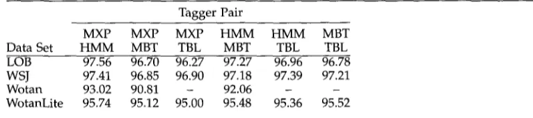
Table 3
Pairwise agreement between the base taggers. For each base tagger pair and data set, we list the percentage of tokens in the test set on which the two taggers select the same tag.
Tagger Pair
MXP MXP MXP HMM HMM MBT
Data Set HMM MBT TBL MBT TBL TBL
LOB 97.56 96.70 96.27 97.27 96.96 96.78
WSJ 97.41 96.85 96.90 97.18 97.39 97.21
Wotan 93.02 90.81 - 92.06 - -
WotanLite 95.74 95.12 95.00 95.48 95.36 95.52
(WSJ a n d WotanLite) MXPOST is the better s y s t e m . In all cases, except the difference b e t w e e n MXP a n d H M M o n LOB, the differences are statistically significant (p K 0.05, M c N e m a r ' s c h i - s q u a r e d test).
We can also see f r o m these results that WSJ, a l t h o u g h it is a b o u t the s a m e size as LOB, a n d h a s a smaller tagset, h a s a h i g h e r difficulty level t h a n LOB. We s u s p e c t that a n i m p o r t a n t r e a s o n for this is the inconsistency in the WSJ a n n o t a t i o n (cf. R a t n a p a r k h i 1996). We e x a m i n e this effect in m o r e detail below. The E i n d h o v e n c o r p u s , b o t h w i t h W o t a n a n d WotanLite tagsets, is y e t m o r e difficult, b u t h e r e the difficulty lies m a i n l y in the c o m p l e x i t y of the tagset a n d the large p e r c e n t a g e of u n k n o w n w o r d s in the test sets. We see that the r e d u c t i o n in the c o m p l e x i t y of the tagset f r o m W o t a n to WotanLite leads to a n e n o r m o u s i m p r o v e m e n t in accuracy. This g r a n u l a r i t y effect is also e x a m i n e d in m o r e detail below.
4.2 Base Tagger Agreement
v a n Halteren, Zavrel, and Daelemans Combination of Machine Learning Systems
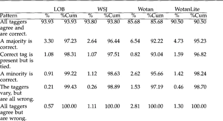
T a b l e 4
The presence of various tagger (dis)agreeement patterns for the four d a t a sets. In a d d i t i o n to the percentage of the test sets for which the pattern is observed (%), we list the cumulative percentage (%Cum).
LOB WSJ Wotan WotanLite
Pattern % % C u m % %Cure % %Cure % %Cum
All taggers 93.93 93.93 93.80 93.80 85.68 85.68 90.50 90.50 agree and
are correct.
A majority is 3.30 97.23 2.64 96.44 6.54 92.22 4.73 95.23 correct.
Correct tag is 1.08 98.31 1.07 97.51 0.82 93.04 1.59 96.82 present b u t is
tied.
A minority is 0.91 99.22 1.12 98.63 2.62 95.66 1.42 98.24 correct.
The taggers 0.21 99.43 0.26 98.89 1.53 97.19 0.46 98.70 vary, b u t
are all wrong.
All taggers 0.57 100.00 1.11 100.00 2.81 100.00 1.30 100.00 agree but
are wrong.
It is i n t e r e s t i n g to s e e t h a t a l t h o u g h t h e g e n e r a l a c c u r a c y for WSJ is l o w e r t h a n for LOB, t h e i n t e r t a g g e r a g r e e m e n t for WSJ is o n a v e r a g e h i g h e r . It w o u l d s e e m t h a t t h e l e s s c o n s i s t e n t t a g g i n g f o r WSJ m a k e s it e a s i e r for all s y s t e m s to fall i n t o t h e s a m e t r a p s . T h i s b e c o m e s e v e n c l e a r e r w h e n w e e x a m i n e t h e p a t t e r n s o f a g r e e m e n t a n d see, for e x a m p l e , t h a t t h e n u m b e r o f t o k e n s w h e r e all t a g g e r s a g r e e o n a w r o n g t a g is p r a c t i c a l l y d o u b l e d .
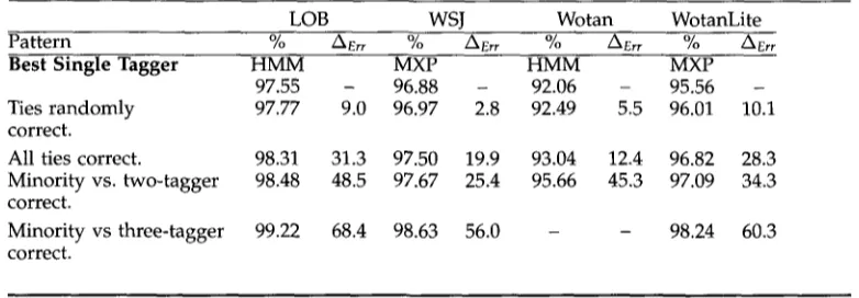
T h e a g r e e m e n t p a t t e r n d i s t r i b u t i o n e n a b l e s u s to d e t e r m i n e l e v e l s o f c o m b i n a t i o n q u a l i t y . Table 5 lists b o t h t h e a c c u r a c i e s o f s e v e r a l i d e a l c o m b i n e r s (%) a n d t h e e r r o r r e d u c t i o n i n r e l a t i o n to t h e b e s t b a s e t a g g e r for t h e d a t a set i n q u e s t i o n (/~Err). 22 F o r e x a m p l e , o n LOB, " A l l ties c o r r e c t " p r o d u c e s 1,941 e r r o r s ( c o r r e s p o n d i n g to a n a c c u r a c y o f 98.31%), w h i c h is 31.3% l e s s t h a n H M M ' s 2,824 e r r o r s . A m i n i m a l l e v e l of c o m b i n a t i o n a c h i e v e m e n t is t h a t a m a j o r i t y o r b e t t e r w i l l l e a d to t h e c o r r e c t t a g a n d t h a t ties a r e h a n d l e d a p p r o p r i a t e l y a b o u t 50% o f t h e t i m e f o r t h e (2-2) p a t t e r n a n d 25% for t h e ( 1 - 1 - 1 - 1 ) p a t t e r n (or 33.3% for t h e ( 1 - 1 - 1 ) p a t t e r n for W o t a n ) . I n m o r e o p t i m i s t i c s c e n a r i o s , a c o m b i n e r is a b l e to s e l e c t t h e c o r r e c t t a g i n all t i e d c a s e s , o r e v e n i n c a s e s w h e r e a t w o - o r t h r e e - t a g g e r m a j o r i t y m u s t b e o v e r c o m e . A l t h o u g h t h e p o s s i b i l i t y o f o v e r c o m i n g a m a j o r i t y is p r e s e n t w i t h t h e a r b i t e r t y p e c o m b i n e r s , t h e s i t u a t i o n is r a t h e r i m p r o b a b l e . A s a r e s u l t , w e o u g h t to b e m o r e t h a n s a t i s f i e d if a n y c o m b i n e r s a p p r o a c h t h e l e v e l c o r r e s p o n d i n g to t h e p r o j e c t e d c o m b i n e r w h i c h r e s o l v e s all ties correctly. 23
22 We express the error reduction in the form of a percentage, i.e., a relative measure, instead of by an absolute value, because we feel this is the more informative of the two. After all, there is a vast difference between an accuracy improvement of 0.5% from 50% to 50.5% (a /KEr r of 1%) and one of 0.5% from 99% to 99.5% (a /KErr of 50%).
[image:17.468.38.405.111.311.2]Computational Linguistics Volume 27, N u m b e r 2
Table 5
Projected accuracies for increasingly successful levels of combination achievement. For each level we list the accuracy (%) a n d the percentage of errors made by the best i n d i v i d u a l tagger
that can be corrected b y combination (AEFr).
LOB WSJ Wotan WotanLite
Pattern % AEr r % AEr r % AEr r % AEr r
Best Single Tagger H M M MXP H M M MXP
97.55 - 96.88 - 92.06 - 95.56 -
Ties r a n d o m l y 97.77 9.0 96.97 2.8 92.49 5.5 96.01 10.1
correct.
All ties correct. 98.31 31.3 97.50 19.9 93.04 12.4 96.82 28.3
Minority vs. two-tagger 98.48 48.5 97.67 25.4 95.66 45.3 97.09 34.3
correct.
Minority vs three-tagger 99.22 68.4 98.63 56.0 - - 98.24 60.3
correct.
Table 6
Accuracies of the combination systems o n all four corpora. For each system we list its accuracy (%) a n d the percentage of errors made b y the best i n d i v i d u a l tagger that is corrected b y the combination system (A~,).
LOB WSJ Wotan WotanLite
% AErr % AErr % AErr % AErr
Best Single Tagger H M M MXP H M M MXP
97.55 - 96.88 - 92.06 - 95.56
Voting
Majority 97.76 9.0 96.98 3.1 92.51 5.7 96.01 10.1
TotPrecision 97.95 16.2 97.07 6.1 92.58 6.5 96.14 12.9
TagPrecision 97.82 11.2 96.99 3.4 92.51 5.7 95.98 9.5
Precision-Recall 97.94 16.1 97.05 5.6 92.50 5.6 96.22 14.8
TagPair 97.98 17.8 97.11 7.2 92.72 8.4 96.28 16.2
Stacked Classifiers
WPDV(Tags) 98.06 20.8 97.15 8.7 92.86 10.1 96.33 17.2
WPDV(Tags+Word) 98.07 21.4 97.17 9.3 92.85 10.0 96.34 17.5
WPDV(Tags+Context) 98.14 24.3 97.23 11.3 93.03 12.2 96.42 19.3
MBL(Tags) 98.05 20.5 97.14 8.5 92.72 8.4 96.30 16.7
MBL(Tags+Word) 98.02 19.2 97.12 7.6 92.45 5.0 96.30 16.6
MBL(Tags+Context) 98.10 22.6 97.11 7.2 92.75 8.7 96.31 16.8
DecTrees(Tags) 98.01 18.9 97.14 8.3 92.63 7.2 96.31 16.8
DecTrees(Tags+Word) -* . . . .
DecTrees(Tags+Context) 98.03 19.7 97.12 7.7 - - 96.26 15.7
Maccent(Tags) 98.03 19.6 97.10 7.1 92.76 8.9 96.29 16.4
Maccent(Tags+Word) 98.02 19.3 97.09 6.6 92.63 7.2 96.27 16.0
Maccent(Tags+Context) 98.12 23.5 97.10 7.0 93.25 15.0 96.37 18.2
c5.0 was not able to cope with the large a m o u n t of data involved in all Tags+Word experiments a n d the Tags+Context experiment with Wotan.
4.3 R e s u l t s o f C o m b i n a t i o n
[image:18.468.45.436.111.247.2] [image:18.468.48.429.297.553.2]van Halteren, Zavrel, and Daelemans Combination of Machine Learning Systems
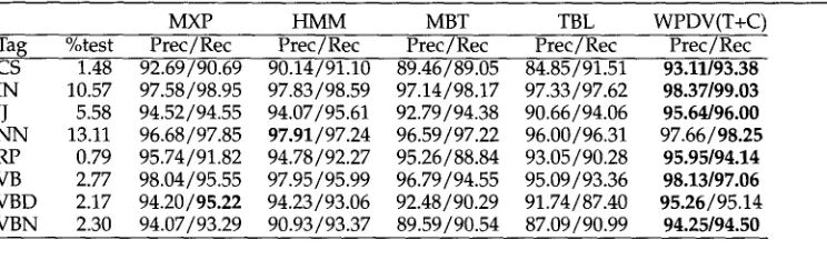
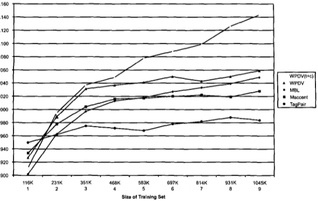
Although the combiners generally fall short of the "All ties correct" level (cf. Table 5), even the most trivial voting system (Majority), significantly outperforms the best individual tagger on all data sets. Within the simple voting systems, it appears that use of more detailed voting weights does not necessarily lead to better results. TagPrecision is clearly inferior to TotPrecision. On closer examination, this could have been expected. Looking at the actual tag precision values (see Table 9 below), we see that the precision is generally more dependent on the tag than on the tagger, so that TagPrecision always tends to select the easier tag. In other words, it uses less specific rather than more specific information. Precision-Recall is meant to correct this behavior by the involvement of recall values. As intended, Precision-Recall generally has a higher accuracy than TagPrecision, but does not always improve on TotPrecision. Our previously unconfirmed hypothesis, that arbiter-type combiners would be able to outperform the gang-type ones, is now confirmed. With the exception of several of the Tags+Word versions and the Tags+Context version for WSJ, the more sophisticated modeling systems have a significantly better accuracy than the simple voting systems on all four data sets. TagPair, being somewhere between simple voting and stacking, also falls in the middle where accuracy is concerned. In general, it can at most be said to stay close to the real stacking systems, except for the cleanest data set, LOB, where it is clearly being outperformed. This is a fundamental change from our earlier experiments, where TagPair was significantly better than MBL and Decision Trees. Our explanation at the time, that the stacked systems suffered from a lack of training data, appears to be correct. A closer investigation below shows at which amount of training data the crossover point in quality occurs (for LOB).
Another unresolved issue from the earlier experiments is the effect of making word or context information available to the stacked classifiers. With LOB and a single 114K tune set (van Halteren, Zavrel, and Daelemans 1998), both MBL and Decision Trees degraded significantly when adding context, and MBL degraded when adding the
w o r d . 24 With the increased amount of training material, addition of the context gener- ally leads to better results. For MBL, there is a degradation only for the WSJ data, and of a much less pronounced nature. With the other data sets there is an improvement, significantly so for LOB. For Decision Trees, there is also a limited degradation for WSJ and WotanLite, and a slight improvement for LOB. The other two systems appear to be able to use the context more effectively. WPDV shows a relatively constant significant improvement over all data sets. Maccent shows more variation, with a comparable improvement on LOB and WotanLite, a very slight degradation on WSJ, and a spec- tacular improvement on Wotan, where it even yields an accuracy higher than the "All ties correct" level. 25 Addition of the word is still generally counterproductive. Only WPDV sometimes manages to translate the extra information into an improvement in accuracy, and even then a very small one. It would seem that vastly larger amounts of training data are necessary if the word information is to become useful.
5. C o m b i n a t i o n in Detail
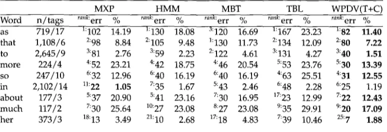
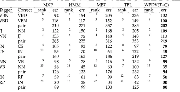
The observations about the overall accuracies, although the most important, are not the only interesting ones. We can also examine the results of the experiments above in more detail, evaluating the results of combination for specific words and tags, and
24 Just as in the c u r r e n t e x p e r i m e n t s , the Decision Tree s y s t e m c o u l d n o t cope w i t h the a m o u n t of d a t a w h e n t h e w o r d w a s a d d e d .