A. Process Review



Abstract—This research focuses on the lapping process

optimization by designed experiments and response surface methods. The lapping process intends to introduce a finely ground flat on disk clamp, the lapping process will remove material from the disk contact radius and provide the desired dimension of the surface. The lapping plate is produced by cubic boron nitride materials. Its mechanism and characteristics are very complicated to conduct and investigate. In addition, the two-level factorial design was applied to a preliminary study, the analysis of variance was performed to determine the optimal combination of process variables which consist of lapping time, lapping speed, downward pressure and charging pressure. The desirability function approach of the nominal-the-best was used to compromise the multiple responses of material removal, lap width and clamp force into single response called the overall desirability (D). Firstly, the multiple regression models were developed from the statistically significant parameters. Secondly, the multi regression model in forms of the path of steepest ascent moved the region of experimental region toward the design point with the maximal D level. After the path of steepest ascent deteriorated the modified simplex method was integrated to drive the process achieving the optimal condition. The experimental results showed that there is a significant D increase to the level of 0.92, approximately 50% when compared to the current operating condition. The optimal condition of process variables which consist of lapping time, lapping speed, downward pressure and charging pressure are 49 sec., 26 rpm, 6.9 psi and 7.7 psi, respectively.

Index Terms—Desirability Function Approach, Modified

Simplex Method, Steepest Ascent Method, Surface Lapping Process.

I. INTRODUCTION

APPING process is the process which a material is precisely removed from a work piece (or specimen) to produce a desired dimension, surface finish or shape. A process of lapping has been applied to a wide range of materials and applications, ranging from metals, glass, optics, semiconductors and ceramics. Typical examples are finishing of various components used in the aerospace, automotive, hard disks and its components, mechanical seal,

Manuscript received November 16, 2012; revised November 29, 2012. This work was supported by the Higher Education Research Promotion and National Research University Project of Thailand, Office of the Higher Education Commission. The authors wish to thank the Faculty of Engineering, Thammasat University, THAILAND for the financial support.

*Sitthikorn DUANGKAEW is with the Industrial Statistics and Operational Research Unit (ISO-RU), Department of Industrial Engineering, Faculty of Engineering, Thammasat University, 12120, THAILAND, [Phone: 662-564-3002-9; Fax: 662-564-3017; e-mail: [email protected], [email protected]]

Pongchanun LUANGPAIBOON is an Associate Professor, ISO-RU, Department of Industrial Engineering, Faculty of Engineering, Thammasat

fluid handling, and many other precision engineering industries. Lapping processes are used to produce dimensionally accurate specimens to high tolerances (generally less than 2.5 µm uniformity). The lapping plate will rotate at the low speed, less than 80 rpm, and the mid-range abrasive particle of 5-20 µm is typically used [1].

The material removal of work pieces is the main requirement of lapping to meet the process specification including a surface lap width and a desired clamp force. In order to maintain the reliability and lifetime of the produced work piece, it is essential to improve the machining process by optimizing both the lapping process efficient and the consideration of the process parameter influences with surface lap width and clamp force according to customer specifications. The initial of material removal, surface lap width and clamp force have somewhat different values on the mean and standard deviation (Stdev), ranging from 1.384 mm3 _{for material removal, 0.76 mm for surface lap}

width and 26.59 kgf for the clamp force as shown in Table I.

TABLEI

QUALITY CHARACTERISTICS ON THE CURRENT OPERATING CONDITION Response variable Mean Stdev Process requirement Material removal 1.384 0.134 1.0 ± 0.75 mm3

Response variable Mean Stdev Customer requirement Surface lap width 0.765 0.027 0.65 ± 0.20 mm Clamp force 26.59 0.432 28.0 ± 3.0 kgf

II. SURFACE LAPPING PROCESS A. Process Review

Single side lapping is the most frequently used machining process for producing the desired dimension.The advantages of this type of lapping are that many pieces can be machined at one time and beside this, the work holding is very simple, cut rates are consistent and close accuracies are inherent with the process. The machines used in this lapping have a rotating annular-sharped lap plate and work pieces are placed on the flat rotating wheel as shown in Fig. 1. Lapping mainly includes a lap plate, lapping fluid and conditioning ring [2]. Lap plates are made of cubic boron nitride (CBN) with the size of 20 µm, hexagonal tiles of 92% minimal coverage. Lapping fluid is with the cutting fluid Alpha-2, conditioning plate with Al2O3 grit size#220.

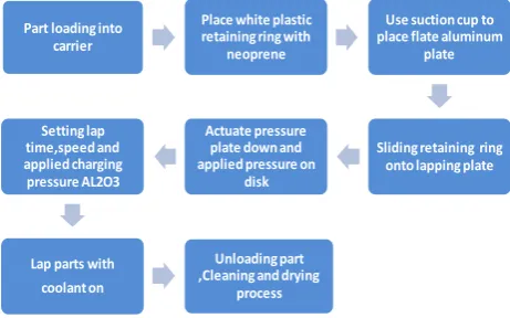
The lapping process consists of four operation steps as shown in Fig. 2. After the part loading into carrier then place a white plastic for retaining ring around parts and template including a neoprene. A suction cup is performed to place a flat aluminum plate on a top of neoprene. The

Surface Lapping Process Improvement via Steepest

Ascent Method Based on Factorial and Simplex Designs

Sitthikorn Duangkaew* and Pongchanun Luangpaiboon, Member, IAENG

lapping plate then actuate the pressure plate down. The main process is to lap a part with the coolant on and simultaneously apply the pressure on a disk, charge Al2O3

[image:2.595.59.277.119.258.2]

pressure, speed up the lapping plate and lapping time. The final steps are to unload the part, clean and dry [3-4].

Fig. 1. Schematic Single Side Lapping Process [2]

Part loading into 

carrier

Place white plastic 

retaining ring with 

neoprene 

Use suction cup to 

place flate aluminum 

plate

Sliding retaining  ring 

onto lapping plate Actuate pressure 

plate down and 

applied pressure on 

disk 

Setting lap 

time,speed and 

applied charging 

pressure AL2O3 

Lap parts with 

coolant on

Unloading part 

,Cleaning and drying 

[image:2.595.47.278.304.448.2]

process

Fig. 2. Surface Lapping Process

B. Lapping Process Variables

After brainstorming via teams who work for the lapping process e.g. advance process development engineer, process engineer, product engineer and quality engineer, the key controllable process variables influencing the lapping characteristics include (1) lapping time (2) lapping speed (3) downward pressure and (4) charging Al2O3 pressure(Table

II).

TABLEII

THE FOUR PROCESS VARIABLES AND THEIR TYPE

Symbol Process variable Type

X1 Lapping time Quantitative

X2 Lapping speed Quantitative

X3 Downward pressure Quantitative

X4 Charging pressure Quantitative

C. Lapping Process’s Quality Measurements

The responses of interest are the material removal (MR), lap width and clamp force. The material removal (MR) is compared with the process requirement specification, the lap width and clamp force are measured and compared with customer requirement specifications. The process and customer specification are required to meet their targets.

III. LAPPING PROCESS OPTIMIZATION METHOD Response surface methodology (RSM) is one of the modeling and optimization approaches currently in wide spread applications in describing the performance of the manufacturing process and finding the optimum of a response of interest. RSM is a collection of mathematical and statistical techniques that are benefit for modeling and analyzing problems in which a response of interest are affected by some process variables and the objective is to optimize the response [5-6]. If all process variables are assumed to be measurable, the response surface can be determined by the regression analyses. In product or process improvement, however, it is quite simple that there are many responses of interest. In this case, determination of optimal operating conditions on the process variables would require simultaneous consideration of all the responses or a multiple response problem. There are three stages for solving the multiple response problems which consist of data collection, model building, and optimization.

A. Desirability Function

The desirability function approach transforms an estimated response (e.g., the ith estimated response of ŷi) into a scale-free value, called a desirability (denoted as

ˆ ( ( ))

i i

d y x for ŷi). The values are between 0 and 1, and increase as the corresponding response values becomes more desirable. The overall desirability D, another value between 0 and 1, is defined by combining the individual desirability values (i.e.,d y xi( ( ))ˆi ’s) [7]. Then, the optimal setting is

determined by maximizing D. In this research, the desirability function for a nominal-the-best (NTB) type response is defined as

max max

?

0 if ( ) ( ) ,

ˆ ( ) _ˆ

if ( ) ,

ˆ ( ( ))

ˆ ( ) _ˆ

if ( ) ,

1

min max

i i i i

si min

min min

i i

i i i

min min

i i

i i _ti

max

max

i i

i i i

max

i i

y x Y or y x Y

y x Y

Y y x T

T Y

d y x

Y y x

T y x Y

Y T

 

   _{ }

 _ 

 



   _{ }

 _ 

 

max

ˆ

if min ( ) ,

i i i

T y x T

        

 _{ }



; where d y xi( ( ))ˆi is the desirability function of ŷi(x)

, min i

Y and max

i

Y are respectively, the lower and upper bounds on the response. min

i

T and max i

T ( min

i

T ≤ max

i

T ) are, respectively, the lower and upper targets of the response.

i

sandt_i are the parameters that determine the shape of ˆ

( ( ))

i i

d y x : if s_i(or t_i) = 1, the shape is linear; if s_i(or t_i) >1,convex; and if 0 <s_i(or t_i) < 1, concave. It should be noted that, if min

i

T = max

i

T , the trapezoidal desirability function reduces to a triangular one.

In this research, defined s_i and t_i equal to 1, the shape is linear, and y1 is the response of material removal (MR). The

min i

Y = 0.25 and max i

Y = 1.75 are respectively, min i

T = 0.90 and max

i

T = 1.10 are respectively, d y x1( ( ))ˆ1 is the desirability

function of y1 which is defined as

1 1 1 1 1 1 1 1 1 ?

0 if ( ) 0.25 ( ) 1.75, ˆ ( ) 0.25 _{if 0.25 ˆ( ) 0.90,}

0.90 0.25 ˆ

( ( ))

ˆ

1.75 ( ) _ˆ

if 1.10 ( ) 1.75, 1.75 1.10

ˆ

1 if 0.90 ( ) 1.10,

y x or y x

y x _{y x}

d y x

y x y x y x     _  _{ }       _{ }    _{ } 

The actual response of y2 is the response of lap width. Yimin

and max i

Y are 0.50 and 0.85, respectively. min i

T and max i

T are

0.625 and 0.675, respectively. d y x₂( ( ))ˆ₂ is the desirability function of y2 which is defined as

                      , 675 . 0 ˆ 625 . 0 if 1 , 85 . 0 ˆ 675 . 0 if 675 . 0 85 . 0 ˆ 0.85 , 625 . 0 ˆ 45 . 0 if 45 . 0 625 . 0 45 . 0 ˆ , 85 . 0 ˆ 45 . 0 ˆ if 0 )) ( ˆ ( (x) y (x) y (x) y (x) y (x) y (x) y or (x) y x y d 2 2 2 2 2 2 2 2 2

The actual response of y3 is the response of lap width. Yimin

and max i

Y are 25.0 and 28.0, respectively. min i

T and max i

T are

27.75 and 28.25, respectively. d y x3( ( ))ˆ3 is the desirability

function of y3 which is defined as

3 3 3 3 3 3 3 3 3 ?

0 if ( ) 25.0 ( ) 31.0,

ˆ ( ) 25.0 _ˆ

if 25.0 ( ) 27.75, 27.75 25.0

ˆ ( ( ))

ˆ 31.0 ( )

ˆ

if 28.25 ( ) 31.0, 31.0 27.75

ˆ

1 if 27.75 ( ) 28.25,

y x or y x

y x

y x d y x

y x y x y x     _  _{ }    _          

B. Steepest Ascent Method (SAM)

The procedure of steepest ascent is that a hyper plane is fitted to the results from the initial 2K _{(fractional) factorial}

designs where K is the number of decision variables. The direction of steepest ascent on the hyper plane is then determined by using principles of least squares and experimental designs. The next run is carried out at a point which is some fixed distance in this direction and further runs are carried out by continuing in this direction until no further increase in yield is noted. When the response first decreases another 2K _{design is carried out, centred on the}

preceding design point. A new direction of steepest ascent is estimated from this latest experiment. Provided at least one of the coefficients of the hyper plane is statistically significantly different from zero, the search continues in this direction. Moreover, the boundary limitations of the process variables are also determined as model constraints [8].

C. Modified Simplex Method (MSM)

A simplex is a K-dimensional polyhedron with K+l vertices, where K is the number of decision variables for optimisation or the dimension of the search space. This sequential optimum search is based on moving away from the experiment with the worst result in a simplex consisting of K+1 experiments [9]. The objective of the sequential simplex method is to drive the simplex toward the region of

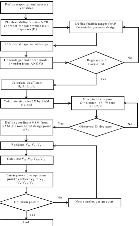
the factor space which is of optimal response. The algorithmic details are as follows. The subsequent vertex is projected with a preset reflection coefficient to the centroid of the hyperface formed by the remaining simplex points a direction opposite from the worst vertex. The new symmetrical simplex consists of one new point and m design points from the previous simplex or discarding the worst point and replacing it with a new point. Repetition of simplex reflection and response measurement form the basis for the most elementary simplex algorithm. Many modifications to the original simplex algorithm have been developed. The details of sequential procedures for setting up the optimum value via a relationship of significant parameters and responses are depicted in Fig. 3.

D ef in e respon ses and p rocess v ariab les

Th e d esirab ility f un ctio n N TB ap p ro ach fo r comp romise m ulti

resp o n ses (D )

2k_{f acto rial exp eriment d esign}

G en erate gen eral lin ear m o del 1st_{o rd er f rom A N O VA}

Calcu late co efficient ß0,ß1,ß2 ...ßk

D ef in e feasib le ran ges f or 2k

f acto rial exp erim ant d esign

Regressio n ? Lack o f f it.

C alcu late step size ? X b y SA M m eth o d

M o v e to n ew regio n D = Cen ter - n ? W h ere

n =1 ,2 ,3 ?

N ew sim p lex d esign p oint D ef in e coo rdinate M SM f ro m

SA M ,th e n u m b er of d esign p o int

K+1 O b serv ed D d ecrease

Calcu late VR,VE, VCR,VC L

O p tim u m p o int ?

En d N o Y es Y es N o Y es N o Ran k in g VH,VS, VL

D riv in g to w ard to o ptim um p o in t b y reflect VL to VR ,

VE,VC R,VC L

[image:3.595.309.549.226.614.2]

Fig. 3 Flow Chart of the Steepest Ascent Method Based on Factorial and Simplex Designs

IV. EXPERIMENT RESULT AND ANALYSIS

The process of lapping was characterized by individually computing the estimated effect in each process variables on the response via screening experiments. The experimental results and analyses to determine the statistically significant effects of four process variables of the lapping time (X1),

lapping speed (X2), downward pressure (X3) and charging

pressure (X4) are applied via the feasible ranges, the current

TABLEIII

PROCESS VARIABLES,FEASIBLE RANGES AND CURRENT LEVELS Process Variables Feasible Ranges Current Unit

Lower Upper

X1 40 60 60 sec.

X2 30 40 30 rpm

X3 8.0 12.0 8.0 psi

X4 8.0 12.0 8.0 psi

In this step, the objective of using a factorial experiment design is to analyze both main and interaction effects for all process variables. The 24 _{experimental designs with two}

replicates provide 32 treatments. The low and high levels were selected cover the values of feasible ranges from the actual operating condition. The material removal, lap width and clamp force were measured from an average value and an estimated responses were transformed into a scale free, denoted as d y x₁( ( ))ˆ₁ for y1 (material removal), d y x2( ( ))ˆ2 for y2

(lap width) and d y x3( ( ))ˆ3 for y3 (clamp force). It is the value

between 0 and 1 and increases as the corresponding response value becomes more desirable.

The overall desirability D is defined by combining the individual desirability of d y x1( ( ))ˆ1 , d y x2( ( ))ˆ2 and d y x3( ( ))ˆ3

values then the optimal setting is determined by maximizing D. By using a general linear model from the analysis of variance (ANOVA), sources of variations focusing on the main and interaction effects and their P-value are shown Table IV. The statistically significant process variables via main effect analysis consist of X1, X2, X3 and X4 as P-value

is less than or equal to 0.05 and the interaction effects of X1*X3 and X2*X3 are also statistically significant at the 95%

confidence interval.

On the first scenario, the method of steepest ascent is then applied for statistically significant quantitative process variables of X1, X2, X3 and X4 to determine the most

preferable fitted equation of associated process variables to the overall desirability D as shown in Table V. The relationship of the process variables and the compromise response of D in terms of the path of steepest ascent are as followed:

D = 0.592 - 0.172 X1 - 0.114 X2 - 0.0788 X3 – 0.0366 X4

TABLEIV

SOURCES OF VARIATION FOCUSING ON THE MAIN AND INTERACTION EFFECTS AND THEIR P-VALUE

Source of variance P-value for D

X1 0.000

X2 0.000

X3 0.000

X4 0.025

X1* X2 0.085

X1* X3 0.004

X1* X4 0.864

X2* X3 0.011

X2* X4 0.627

X3* X4 0.306

TABLEV

REGRESSION MODEL INCLUDING ITS SIGNIFICANT COEFFICIENTS AND ANOVATABLE

Predictor Coef SE Coef T P-value

Constant 0.592 0.01938 30.54 0.000

X1 -0.17214 0.01938 -8.88 0.000

X2 -0.11412 0.01938 -5.89 0.000

X3 -0.07880 0.01938 -4.07 0.000

X4 -0.03664 0.01938 -1.89 0.070

Source DF SS MS F P-value

Regression 4 1.60663 0.40166 33.4 0.000 Residual Error 27 0.32466 0.01202

Total 31 1.93129

In order to move the center of 24 _{experiment design to get}

the maximal level of D, the proper coefficients are determined via the ratio of X1: X2: X3: X4 equalling

0.17214: 0.11412: 0.0788: 0.03664. It means that the 0.17214 units is moving in the direction of X1, 0.11412

units in the direction of X2 , 0.0788 units in the direction of

X3 and 0.03664 units in the direction of X4 and all are in

coded unit data. The coefficients for all process variables were measured by transforming into the natural unit to get 3.84 for X1, 1.27 for X2, 0.35 for X3 and 0.16 for X4. In this

research the step size of 0.50 is selected. The results on the path of steepest ascent determine the near optimal values of process variables as shown in Table VI and Fig. 4.

TABLEVI

THE NEW LEVELS OF PROCESS VARIABLES ALONG WITH OVERALL DESIRABILITY OF D

Step size Process variables Desirability

X1 X2 X3 X4 D

Center 60 30 8.0 8.0 0.455

Center-∆ 56 28 7.5 8.0 0.582

Center-2∆ 52 26 7.5 7.5 0.788

Center-3∆ 48 26 7.0 7.5 0.873

Center-4∆ 45 24 6.5 7.5 0.834

Center-5∆ 41 24 6.5 7.0 0.750

Center-5∆

Center-4∆

Center-3∆

Center-2∆

Center-∆

Center

1.0

0.9

0.8

0.7

0.6

0.5

0.4

0.3

0.2

Steepest Ascent Point

D

e

sir

a

b

ilit

y

[image:4.595.46.287.614.775.2]

d1 : Meterial Removal d2 : Lap width d3 : Clamp force D : Overall Desirability Desirability

From the Table VI, after the fourth step, the direction brings a decrease of the overall desirability D. It can be concluded that the direction of process variables to be changed in order to achieve an increase of the overall desirability is as followed: lapping time (X1) of 48 sec.,

lapping speed (X2) of 26 rpm, downward pressure (X3) of

7.0 psi and charging pressure (X4) of 7.5 psi.

On the second scenario, the modified simplex method is then applied to drive the region of process variables to an optimal response. Firstly, define the coordinate of the starting design point. The number of trials equal to K+1, where k is the number of process variables. In this study, K equals to 4 or the number of the total starting design points is 5 as shown in Table VII. All of these were selected from the steepest ascent path and ranked to VH, VS3, VS2, VS1 and

VL. Secondly, the MSM is to drive toward to the optimum

point by reflecting VL to a new design point of VR and

observe its response.

V_R P (PV )_L

, where P is the centroid of the remaining vertices except VL. If the observed VR is better than VL but worse than VS

the VCRand VCL were selected to be the new simplex. V_{C R} P 0.5(PV )_L

V_{C L} P 0.5(PV )_L

TABLEVII

THE INTEGRATION OF MSM AND SAM DESIGN POINTS

Vertex X1 X2 X3 X4 D Rank

1 48 26 7.0 7.5 0.87 VH

2 45 25 6.5 7.5 0.83 VS3

3 52 27 7.5 7.5 0.79 VS2

4 41 24 6.5 7.0 0.75 VS1

5 56 29 7.5 8.0 0.58 VL1

P 47 26 6.8 7.4

VR1 37 22 6.2 6.8 0.71

VE 27 19 5.6 6.1 -

VCR1 42 24 6.5 7.0 0.81

VCL1 51 27 7.2 7.7 0.84

TABLEVIII

THE MASSIVE CONTRACTION OF PROCESS VARIABLES FROM THE MSM

Vertex X1 X2 X3 X4 D Rank

1 48 26 7.0 7.5 0.87 VH

2 51 27 7.2 7.7 0.84 VS3

3 45 25 6.5 7.5 0.83 VS2

4 42 24 6.5 7.0 0.81 VS1

5 41 24 6.5 7.0 0.75 VL

P 47 25 6.8 7.4

VR 52 27 7.1 7.8 0.78

VE 58 28 7.4 8.3 -

VCR 49 26 6.9 7.7 0.92

VCL 44 25 6.6 7.2 0.88

From the Table VII, VCL1 is greater than VL1, the massive

contraction of process variables will be defined and repeated by a new rank then the VCL1, VCR1 and VL1 were selected

instead of new VS3 and VS1 and VL. The experimental results

can be determined the optimal response based on VCR

(Table VIII). The preferable levels of process variables by integrated approach of steepest ascent and modified simplex methods are summarized in Table IX.

TABLEIX

PREFERABLE LEVELS OF INFLUENTIAL PROCESS VARIABLES FROM THE FIRST AND SECOND SCENARIOS

Process

variables Description

Operating condition Current SAM MSM

X1 Lapping time 60 48 49

X2 Lapping speed 30 26 26

X3 Downward pressure 8.0 7.0 6.9

X4 Charging pressure 8.0 7.5 7.7

From the process settings for all influential process variables in Table IX, the performance after the improvement of two phases can be evaluated from the desirability levels. Based on the confirmation data, it has been found that the average of the responses from the scenarios 1 and 2 is greater than the current operating condition which can be explained by the box-whisker plot (Fig. 5).

(3) MSM (2) SAM

(1) Current 1.0

0.9

0.8

0.7

0.6

0.5

scenario

O

v

e

ra

l D

e

sir

a

b

ili

ty

(

D

)

Box Whisker plot of overall desirability from three scenario

TABLEX

ONE WAY ANOVA:DESIRABILITY VERSUS SCENARIO

Source DF SS MS F P-value

Regression 2 1.5769 0.7884 2239.09 0.000 Residual Error 57 0.0200 0.00035

Total 59 1.5970

Fig. 6. Graphical Comparison for Three Scenarios

0.050 0.025 0.000 -0.025 -0.050

99.9 99 90 50 10 1 0.1

Residual

Pe

rc

en

t

0.9 0.8 0.7 0.6 0.050

0.025

0.000

-0.025

-0.050

Fitted Value

Re

si

du

al

0.04 0.02 0.00 -0.02 -0.04 16

12

8

4

0

Residual

Fr

eq

ue

nc

y

60 55 50 45 40 35 30 25 20 15 10 5 1 0.050

0.025

0.000

-0.025

-0.050

Observation Order

Re

si

du

al

Normal Probability Plot Versus Fits

Histogram Versus Order

[image:6.595.48.546.66.434.2]

Residual Plots for Desirability (D)

Fig. 7. Model Adequacy Checking V. CONCLUSION

In this research there are three responses to be considered in order to achieve their targets. The desirability function for a nominal-the-best was applied to compromise multiple responses with the integration of the steepest ascent method based on factorial designs and the modified simplex method. The experimental results showed the following notes.

1) The material removal (MR) can meet the process specification and achieve the proper lap width dimension from the customer specification. It can be said the proper process specification of material removal can be used to predict the lap width dimension as required by customers. The optimal levels of process variables are the lapping time at 49 sec, lapping speed at 26 rpm, downward pressure at 6.9 psi and charging pressure at 7.7 psi.

2) The improvement of clamp force slightly increases with decreased lapping time, lapping speed, downward pressure and charging pressure. This phenomenon is more noticeable against the direction of material removal to achieve the lap width dimension. It means that there are other process variables with somewhat more influence. For the free-state height, body angle and hardness of work pieces these need to be under a consideration and could be more important to achieve the proper value. The free-state height of work pieces should be recommended to set a bit higher than the current one in order to bring the clamp force to, at least, near the optimal point or its target.

REFERENCES

[1] Lapping & Polishing Basic,Application Laboratory Report 54 .,South

Bay Technology Inc.,pp.1-7,http://www.southbaytech.com/appnotes/ 54

[2] I.D. Marinescu, E. Uhlmann and T.K. Doi, “Handbook of Lapping and Polishing,” Taylor & Francis, Chapter 3, pp. 109-111, 2006. [3] Y. Zhang, “Study and Optimization of D2 Steel Lapping Using a

Tribological Designed Plate,” A Thesis Submitted to the Graduate Faculty as partial fulfillment of the requirements, Master of Science Degree in Mechanical Engineering, The University of Toledo, May 2010.

[4] J.D. Kim and M.S. Choi, “A Study on the optimization of cylindrical lapping process for engineering fine-ceramics (Al2O3) by the

statistical design method,” Journal of Materials Processing

Technology, 1994, pp. 368-385.

[5] W. Sayasang and P. Luangpaiboon, “Meandering Improvement of Stealth Laser Dicing Via Mixed Integer Linear Constrained Response Surface Optimization Model,” Operation Research Network of

Thailand International Conference, Sep 2011.

[6] P. Luangpaiboon, (2002), “Process Optimization via Conventional Factorial Designs and Simulated Annealing on the Path of Steepest Ascent for a CSTR”, Proceedings of International Conference in

Operations Research 2002, Klagenfurt University, AUSTRIA, pp.

329-334.

[7] I.J. Jeong and K.J. Kim, “Stochastics and Statistics: An interactive desirability function method to multi response optimization,”

European Journal of operation Research, Vol. 195, 2009, pp.

412-426.

[8] P. Luangpaiboon, Y. Suwanknam and S. Homrossukon, “Constrained Response Surface Optimization for Precisely Atomizing Spraying Process”, IAENG Transactions on Engineering Technologies, Vol. 5, 2010, pp. 286-300. DOI: 10.1063/1.3510555