Eigen Vector Descent and Line Search
for Multilayer Perceptron
Seiya Satoh and Ryohei Nakano
Abstract—As learning methods of a multilayer perceptron (MLP), we have the BP algorithm, Newton’s method, quasi-Newton method, and so on. However, since the MLP search space is full of crevasse-like forms having a huge condition number, it is unlikely for such usual existing methods to perform efficient search in the space. This paper proposes a new search method which utilizes eigen vector descent and line search, aiming to stably find excellent solutions in such an extraordinary search space. The proposed method is evaluated with promising results through our experiments for MLPs having a sigmoidal or exponential activation function.
Index Terms—multilayer perceptron, polynomial network, singular region, search method, line search
I. INTRODUCTION
The search space of a multilayer perceptron (MLP) is reported to be full of like forms such as crevasse-local-minima or a crevasse-gutter having a huge condition number (106 ∼ 1017) [4]. In such an extraordinary space, it will be hard for usual existing search methods to find excellent solutions.
In MLP learning, the BP algorithm is well known as a first-order method, but its learning is usually very slow and will get stuck in crevasse-like forms. Second-order methods, such as Newton’s method and quasi-Newton method, can converge much faster into a local minimum or gutter; however, it will not be easy even for them to find a descending route once they get stuck in a gutter [4].
Recently a new search method [3] has been invented, which directly positions hidden units within input space by numerically analyzing the curvature of the output surface.
This paper proposes another new search method which utilizes eigen vector descent and line search, aiming to stably find excellent solutions in such an extraordinary search space full of crevasse-like forms. Our experiments using sigmoidal MLP and polynomial-type MLP showed that the proposed method worked well for artificial and real data.
II. BACKGROUND
Consider a multilayer perceptron (MLP) havingJ hidden units and one output unit. The MLP output f for the µ-th data point is calculated as below.
f(xµ;w) =w0+ J
∑
j=1
wjz µ j, z
µ j ≡g(w
T jx
µ) (1)
Here w = {w0, wj,wj, j = 1,· · ·, J} denotes a weight vector. Given data {(xµ, yµ), µ = 1,· · ·, N}, we want to
This work was supported in part by Grants-in-Aid for Scientific Research (C) 22500212 and Chubu University Grant 22IS27A.
S. Satoh, and R. Nakano are with the Department of Computer Science, Graduate School of Engineering, Chubu University, 1200 Matsumoto-cho, Kasugai 487-8501, Japan email: [email protected], and [email protected]
find the weight vector that minimizes sum-of-squares error E shown below.
E=1 2
N
∑
µ=1
(fµ−yµ)2, fµ≡f(xµ;w) (2)
A. Existing Search Methods
(1) BP algorithm and Coordinate Descent
The batch BP algorithm is a steepest descent method, and updates weights using the following equations. Hereηtis a learning rate at timet, andg(w)denotes a gradient atw.
wt+1=wt−ηtgt, gt≡g(wt), g(w)≡
∂E
∂w (3)
The so-called BP algorithm is a stochastic descent method which updates weights each time a data point is given. Both BP algorithms are usually very slow and likely to get stuck at points which are not so good.
Coordinate descent method only changes a single weight with the remaining weights fixed. Since the coordinates of weights are orthogonal, the method selects the descent direction among the orthogonal candidates. There are several ways of selecting a suitable coordinate [2].
(2) Newton’s method
The idea behind Newton’s method is that the target func-tion is approximated locally by a quadratic funcfunc-tion, and the method usually converges much faster than first-order methods stated above. The method updates weights using the following equations.
wt+1=wt−H−t1gt,Ht≡H(wt),H(w)≡
∂2E
∂wT∂w (4) HereH(w)denotes the Hessian matrix atw. At a strict local minimumw∗the Hessian matrixH(w∗)is positive definite; however, in a crevasse-like gutter having a huge condition number the positive definiteness and the search direction are in a precarious condition. Moreover, the additional cost of computing the Hessian matrix is required, and Newton’s method may head for a local maximum.
(3) quasi-Newton methods and BPQ
Quasi-Newton methods employ an approximation to the inverse Hessian in place of the true required in Newton’s method. The approximation can be built up by using a series of gradients obtained through a learning process. Let Gt be an approximation to the inverse Hessian, then the search directiondt is given as below.
dt=−Gtgt (5)
search. There are a number of techniques for performing line search [2]. BPQ algorithm [5] employs the BFGS update for calculating the inverse Hessian and the second-order approximation for calculating a step length.
B. Properties of MLP Search Space
(1) local minimum, wok-bottom, gutter, and crevasse Here we review a critical point where the gradient∂E/∂w
of a target functionE(w)gets zero. In the context of mini-mization, a critical point is classified into a local minimum and a saddle. A critical point w0 is classified as a local
minimum when any point w in its neighborhood satisfies E(w0)≤E(w), otherwise is classified as a saddle.
Now we classify a local minimum into a wok-bottom and a gutter [4]. A wok-bottomw0is a strict local minimum where
any point w in its neighborhood satisfiesE(w0)< E(w),
and a gutter is a set of points connected to each other in the form of a continuous subspace where any two pointsw1and
w2in a gutter satisfyE(w1) =E(w2)orE(w1)≈E(w2).
When a point has a huge condition number (say, more than
105), we say the point is in a crevasse. A wok-bottom and a
gutter in a crevasse are called a crevasse-wok-bottom and a crevasse-gutter respectively.
(2) singular region
One of the major characteristics of MLP search space is the existence of singular regions [1], [4], [8]. Here MLP(J) denotes an MLP havingJ hidden units. A singular region is defined as a search subspace where the gradient is equal to zero (∂E/∂w = 0) and the Hessian matrix is not positive definite with at least one eigen value equal to zero. Thus, a singular region is a flat subspace, and points in and around a singular region have a huge condition number.
How is a singular region created? It is known that among MLPs the following causes three types of reducibility [7].
a)wj= 0
b) wj= (wj0,0,· · ·,0)T
c)wj1 =wj2
Based on the above reducibility, a singular region in the search space of MLP(J) is generated by applying the fol-lowing reducible mapping to a local minimum wbJ−1 =
{bu0,buj,ubj, j= 2, ..., J} of MLP(J−1) [1], [4].
b
θJ−1
α
−→ΘbαJ, bθJ−1 β
−→ΘbβJ, bθJ−1 γ −→ΘbγJ
b
ΘαJ ≡ {θJ| w0=bu0, w1= 0,
wj =ubj,wj=ubj, j= 2,· · ·, J} (6)
b
ΘβJ ≡ {θJ| w0+w1g(w10) =ub0,
w1= [w10,0,· · ·,0]T,
wj =ubj,wj=ubj, j= 2,· · ·, J} (7)
b
ΘγJ ≡ {θJ| w0=ub0, w1+w2=ub2,
w1=w2=ub2,
wj =ubj,wj=ubj, j= 3,· · ·, J} (8)
(3) another cause of a huge condition number
As stated above, points in and around a singular region have a huge condition number, which causes stagnation of learning. Moreover, there exists another aspect why MLP search space has points having a huge condition number.
Consider the following simple MLP.
f =w0+xw11 (9)
Let the range of x be (0, 1), and the current values of weights be as w0 = 1 and w11 = 1. When the value of
w0 is incremented by one, the MLP output changes widely
as shown in Fig. 1 (a). Meanwhile, when the value of w11
is similarly incremented by one, the MLP output hardly changes as shown in Fig. 1 (b). As shown in this simple example, the influence over the MLP output differs widely among weights, which may generate points having a huge condition number.
0 0.2 0.4 0.6 0.8 1
0 0.5 1 1.5 2 2.5 3
x
f
f 2+x10
(a)w0is changed from 0 to 1
0 0.2 0.4 0.6 0.8 1
0 0.5 1 1.5 2 2.5 3
x
f
f 1+x11
[image:2.595.314.536.217.313.2](b)w11is changed from 0 to 1
Fig. 1. How the change of a weight influences the output of MLP.
III. EIGENVECTORDESCENT
In a crevasse-gutter usual existing methods will not pro-ceed along the bottom of a gutter, but will try to go down heading for the opposite steep wall, and finally will get stuck around the bottom of the gutter.
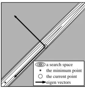
As a robust search method which can proceed along the bottom of a crevasse-gutter, we propose a new method which utilizes a set of eigen vectors to find a desirable search direction even in a crevasse-gutter.
LetH,λm, andvmbe the Hessian matrix, its eigen value, and the corresponding eigen vector, respectively.
Hvm=λmvm (10)
Note that eigen vectors are orthogonal to each other if their eigen values are different. Then, we can expect that one of eigen vectors is almost parallel to the bottom of a crevasse-gutter as shown in Fig. 2.
[image:2.595.359.499.597.742.2]a search space the minimum point the current point eigen vectors
Now that the candidates of the search direction are deter-mined, we consider line search which determines an adequate step length how far the search point should be moved. There are many techniques for line search [2], and the second-order Taylor expansion is sometimes used as line search by curve fitting. Here we consider the third-order approximation as well to deal with a negative curvature.
Letvm,tbe them-th eigen vector of the Hessian matrix at timet; then, the target function Eatwtalong the direction
vm,t is expressed as ψt(η) = E(wt+η vm,t). The third-order Taylor expansion is shown as follows.
ψt(η)≈ψt(0) +ψt0(0)η+
1 2ψ
00
t(0)η 2
+1
6ψ 000
t (0)η 3
(11)
The solution ηt which minimizes the above ψt(η) can be easily obtained by solving the quadratic equation. If we have two solutions positive and negative, we select the positive one. When both solutions are positive, we select the smaller one. Moreover, if we don’t have a positive solution, we employ the second-order Taylor expansion.
Now, we describe the proposed search method, which is called EVD (eigen vector descent). EVD repeats the following basic search cycle until convergence. The basic cycle at time tis shown below.
Basic cycle of EVD :
(step 1) Calculate the Hessian matrix and get all the eigen vectors{vm,t, m= 1,· · ·, M}.
(step 2) Calculate repeatedly the adequate step length ηm,t for each eigen vector vm,t by using the second- or third-order Taylor expansion.
(step 3) Update weights using the suitable search direction
d∗t and its step lengthη∗t.
wt+1 ←− wt+η∗td∗t (12)
Here the pair of d∗t andη∗t is determined based on all the eigen vectors and their step lengths obtained above.
We consider three ways of performing step 3. As the first one, all the eigen vectors are considered as candidates and the pair of eigen vector and its step length which minimizes E is selected as d∗t andηt∗. This is calledEVD1.
As the second one, a linear combination of all the eigen vectors is considered as a single candidate. More specifically,
∑
mηm,tvm,tgives the search direction and step length. This is calledEVD2.
As the third one, all the eigen vectors and the linear combination stated above are considered as candidates, and the best one is selected asd∗t andηt∗. This is calledEVD3.
IV. EXPERIMENTALEVALUATION
The proposed methods are evaluated for MLPs having a sigmoidal or exponential activation function using two artifi-cial data sets and one real data set. The forward calculation of a sigmoidal MLP goes as below.
f =w0+ J
∑
j=1
wjzj, zj =σ(wTjx) (13)
The forward calculation of a polynomial-type MLP goes as shown below. This type of MLP can represent multivariate
polynomials [6]. Note that there is no bias unit in the input layer of this model.
zj = K
∏
k=1
(xk)wjk = exp
(K ∑
k=1
wjklnxk
)
, (14)
f =w0+ J
∑
j=1
wjzj (15)
The proposed methods have six types: EVD1, EVD2, and EVD3 are combined with two kinds of line search using the second- or third-order Taylor expansion. EVD1 (2nd), for example, indicates EVD1 combined with line search using the second-order Taylor expansion. As the existing methods, BP, CD (coordinate descent), and BPQ are combined with two kinds of line search. Thus, BP (2nd), for example, follows the same notation as above.
The basic cycle is repeated until one of the following is satisfied: the step length gets smaller than10−30, the absolute value of any gradient element gets smaller than 10−30, or
the number of sweeps exceeds 20,000. For each data set, learning was performed 100 times changing initial weights. During a learning process we monitor eigen values and the condition number.
100 101 102 103 104
10−30
10−25
10−20
10−15
10−10
10−5
100
105
sweeps
E
(a) BP (2nd)
100 101 102 103 104
10−30
10−25
10−20
10−15
10−10
10−5
100
105
sweeps
E
(b) BPQ (2nd)
100 101 102 103 104
10−30
10−25
10−20
10−15
10−10
10−5
100
105
sweeps
E
[image:3.595.356.497.364.752.2](c) EVD3 (2nd)
A. Sigmoidal MLP for Artificial Data 1
Artificial data 1 was generated for a sigmoidal MLP. The value ofxkwas randomly selected from the range(0,1), and teacher signalywas calculated using the following weights; 500 data points were generated (N = 500).
w0= 5, w1= 10, w1=
1 22 23 24
(16)
Weights are randomly initialized from the range(−1,+1), and the final weights are classified as correct if any difference between the corresponding weights of the original and the final is less than 10−3.
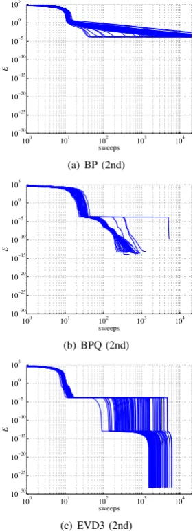
Figure 3 shows how training error E decreased through learning of BP (2nd), BPQ (2nd), and EVD3 (2nd). We can clearly see BP was trapped in the first gutter, and BPQ somehow escaped it but got stuck in the second gutter, while EVD3 (2nd) escaped even the second, reaching the true minimum.
All six types of proposed methods reached the correct weights for all 100 runs. Any existing method, however, didn’t reach the correct weights at all.
0 500 1000
1500 10−15
10−10 10−5 100 105
sweeps
eigenvalues
(a) Eigen Values
0 500 1000 1500 2000
10−30 10−20 10−10 100 1010
sweeps
E
0 500 1000 1500 200010
0
105
1010
1015
1020
condition number
[image:4.595.350.499.330.719.2](b) Condition Numbers
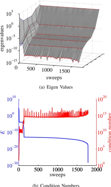
Fig. 4. How Eigen Values and the Condition Number Changed through EVD3 (2nd) Learning of Sigmoidal MLP for Artificial Data 1
Figure 4 shows how eigen values and the condition number changed during learning of EVD3 (2nd). The largest eigen value kept being almost constant through learning, while the smallest one decreased rapidly in an early stage, which reflected the growth of the condition number. That is, the condition number increased from 104 to 1016 in an early stage of learning, and then kept vibrating around1016. Note
also that there is a remarkable tendency that a rapid increase of the condition number occurs simultaneously with a rapid decrease of training errorE. Since the condition number of the final point is around1016, the final point is a
crevasse-wok-bottom.
B. Polynomial-type MLP for Artificial Data 2
Here we consider the following polynomial.
y = 5 + 10x221 x232 x243 (17)
Artificial data 2 was generated for a polynomial-type MLP. The value ofxk was randomly selected from the range(0,1), and teacher signalywas calculated using the above equation; 200 data points were generated (N = 200). The weight initialization and the correctness judgement were performed in the same way as artificial data 1.
Figure 5 shows how error E decreased through learning. Much the same tendency as in artificial data 1 was observed; that is, BP was trapped in the first gutter, BPQ was trapped in the second gutter, while EVD3 escaped these gutters, reaching the correct weights in most runs.
100 101 102 103 104
10−35
10−30
10−25
10−20
10−15
10−10
10−5
100
105
1010
sweeps
E
(a) BP (2nd)
100 101 102 103 104
10−35
10−30
10−25
10−20
10−15
10−10
10−5
100
105
1010
sweeps
E
(b) BPQ (2nd)
100 101 102 103 104
10−35
10−30
10−25
10−20
10−15
10−10
10−5
100
105
1010
sweeps
E
(c) EVD3 (3rd)
Fig. 5. Learning Process of Polynomial-type MLP for Artificial Data 2
[image:4.595.78.259.357.661.2]correct weights at all for all 100 runs. Among EVD1, EVD2, and EVD3, EVD3 performed best as a whole. As for line search, the third-order Taylor expansion worked better than the second-order for this data.
TABLE I
THENUMBER OFSUCCESSES OFPOLYNOMIAL-TYPEMLP LEARNING FORARTIFICIALDATA2 (OUT OF100RUNS)
Method EVD1 EVD2 EVD3 BPQ
Taylor Exp. 2nd 3rd 2nd 3rd 2nd 3rd 2nd 3rd Success Count 37 49 0 80 57 69 0 0
CD BP
2nd 3rd 2nd 3rd
0 0 0 0
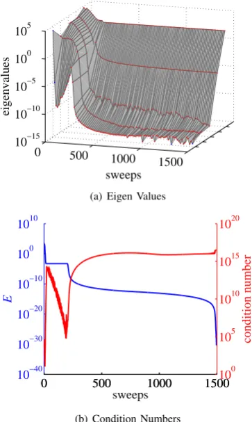
Figure 6 shows how eigen values and the condition number changed during learning of EVD3 (3rd). The largest eigen value kept being almost constant after an early stage, while the smallest one went rapidly down, up and down in an early stage, and then kept being almost constant. After an early stage, the condition number kept being huge around 1016.
Around the 200th sweep a rapid increase of the condition number occurred simultaneously with a rapid decrease of training error E. The final point is a crevasse-wok-bottom.
0 500
1000 1500
10−15 10−10 10−5 100 105
sweeps
eigenvalues
(a) Eigen Values
0 500 1000 1500
10−40 10−30 10−20 10−10 100 1010
sweeps
E
0 500 1000 150010
0
105
1010
1015
1020
condition number
[image:5.595.357.495.177.564.2](b) Condition Numbers
Fig. 6. How Eigen Values and the Condition Number changed through EVD3 (3rd) Learning of Sigmoidal MLP for Artificial Data 2
C. Sigmoidal MLP for Real Data
As real data, ball bearings data (Journal of Statistics Education) (N = 200) was used. The objective is to estimate fatigue(L50) using load(P), the number of balls (Z), and diameter (D). The weight initialization was performed in the
same way as artificial data 1. In this experiment a weak weight decay regularizer (coefficient10−5) was employed.
Figure 7 shows how training error E decreased through learning of BP (2nd), BPQ (2nd), and EVD3 (3rd). BP was trapped in a relatively large error gutter and could not move any further, and BPQ performed relatively well with a few good-quality solutions, while EVD3 (3rd) worked better than BPQ as a whole, finding many better solutions than BPQ could reach.
100 101 102 103 104
105
106
107
sweeps
E
(a) BP (2nd)
100 101 102 103 104
105
106
107
sweeps
E
(b) BPQ (2nd)
100 101 102 103 104
105
106
107
sweeps
E
(c) EVD3 (3rd)
Fig. 7. Learning Process of Sigmoidal MLP for Real Data
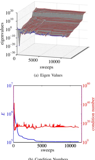
Figure 8 shows how eigen values and the condition number changed during learning of EVD3 (3rd). In this experiment, the largest and the smallest eigen values kept being almost constant after a very early stage. The condition number stayed high between 1015 and1020 throughout the learning
except the beginning.
V. CONCLUSION
[image:5.595.77.259.355.659.2]0 5000
10000 10−30
10−20 10−10 100 1010 1020
sweeps
eigenvalues
(a) Eigen Values
0 5000 10000
105 106 107
sweeps
E
5000 10000 10
0
1020
1040
1060
condition number
[image:6.595.77.259.61.366.2](b) Condition Numbers
Fig. 8. How Eigen Values and the Condition Number changed through EVD3 (3rd) Learning of Sigmoidal MLP for Real Data
we plan to reduce the load for computing eigen vectors, and try to apply our methods to wider variety of data sets to enlarge the applicability.
REFERENCES
[1] K. Fukumizu and S. Amari, “Local minima and plateaus in hierarchical structure of multilayer perceptrons,”Neural Networks, vol. 13, no. 3, pp. 317–327, 2000.
[2] D. G. Luenberger, Linear and Nonlinear Programming, Addison-Wesley Pub.Co., 1973.
[3] R. C.J. Minnett, A. T. Smith, W. C. Lennon Jr. and R. Hecht-Nielsen, “Neural network tomography: network replication from output surface geometry,”Neural Networks, vol.24, no. 5, pp. 484–492, 2011. [4] R. Nakano, S. Satoh and T. Ohwaki, “Learning method utilizing
singular region of multilayer perceptron, ”Proc. of the 3rd International Conference on Neural Computation Theory and Applications (NCTA ’11), pp. 106–111, 2011.
[5] K. Saito and R. Nakano, “Partial BFGS update and efficient step-length calculation for three-layer neural networks,”Neural Computation, vol.9, no. 1, pp. 239–257, 1997.
[6] K. Saito and R. Nakano, “Law discovery using neural networks,”Proc. of 15th International Joint Conf. on Artificial Intelligence (IJCAI), pp. 1078–1083, 1997.
[7] H. J. Sussmann, “Uniqueness of the weights for minimal feedforward nets with a given input-output map,”Neural Networks, vol.5, no. 4, pp. 589–593, 1992.