Modeling Context Words as Regions:
An Ordinal Regression Approach to Word Embedding
Shoaib Jameel and Steven Schockaert School of Computer Science and Informatics
Cardiff University
{JameelS1, SchockaertS1}@cardiff.ac.uk
Abstract
Vector representations of word meaning have found many applications in the field of natural language processing. Word vec-tors intuitively represent the average con-text in which a given word tends to oc-cur, but they cannot explicitly model the diversity of these contexts. Although re-gion representations of word meaning of-fer a natural alternative to word vectors, only few methods have been proposed that can effectively learn word regions. In this paper, we propose a new word embedding model which is based on SVM regression. We show that the underlying ranking in-terpretation of word contexts is sufficient to match, and sometimes outperform, the performance of popular methods such as Skip-gram. Furthermore, we show that by using a quadratic kernel, we can effec-tively learn word regions, which outper-form existing unsupervised models for the task of hypernym detection.
1 Introduction
Word embedding models such as Skip-gram (Mikolov et al., 2013b) and GloVe (Pennington et al., 2014) represent words as vectors of typi-cally around 300 dimensions. The relatively low-dimensional nature of these word vectors makes them ideally suited for representing textual in-put to neural network models (Goldberg, 2016;
Nayak,2015). Moreover, word embeddings have been found to capture many interesting regulari-ties (Mikolov et al., 2013b; Kim and de Marn-effe,2013;Gupta et al.,2015;Rothe and Sch¨utze,
2016), which makes it possible to use them as a source of semantic and linguistic knowledge, and to align word embeddings with visual features
(Frome et al.,2013) or across different languages (Zou et al.,2013;Faruqui and Dyer,2014).
Notwithstanding the practical advantages of representing words as vectors, a few authors have advocated the idea that words may be better repre-sented as regions (Erk,2009), possibly with grad-ual boundaries (Vilnis and McCallum,2015). One important advantage of region representations is that they can distinguish words with a broad mean-ing from those with a more narrow meanmean-ing, and should thus in principle be better suited for tasks such as hypernym detection and taxonomy learn-ing. However, it is currently not well understood how such region based representations can best be learned. One possible approach, suggested in ( Vil-nis and McCallum,2015), is to learn a multivari-ate Gaussian for each word, essentially by requir-ing that words which frequently occur together are represented by similar Gaussians. However, for large vocabularies, this is computationally only feasible with diagonal covariance matrices.
In this paper, we propose a different approach to learning region representations for words, which is inspired by a geometric view of the Skip-gram model. Essentially, Skip-gram learns two vectors pw and p˜w for each word w, such that the
prob-ability that a word c appears in the context of a target word t can be expressed as a function of pt·p˜c(see Section 2). This means that for each
threshold λ ∈ [−1,1]and context word c, there is a hyperplane Hc
λ which (approximately)
sepa-rates the words tfor whichpt·p˜c ≥ λfrom the
others. Note that this hyperplane is completely de-termined by the vectorp˜cand the choice ofλ. An
illustration of this geometric view is shown in Fig-ure1(a), where e.g. the wordcis strongly related toa(i.e. ahas a high probability of occurring in the context ofc) but not closely related tob. Note in particular that there is a half-space containing those words which are strongly related toa(w.r.t.
a given thresholdλ).
Our contribution is twofold. First, we empir-ically show that effective word embeddings can be learned from purely ordinal information, which stands in contrast to the probabilistic view taken by e.g. Skip-gram and GloVe. Specifically, we propose a new word embedding model which uses (a ranking equivalent of) max-margin constraints to impose the requirement that pt·p˜c should be
a monotonic function of the probability P(c|t) of seeing c in the context of t. Geometrically, this means that, like Skip-gram, our model asso-ciates with each context word a number of paral-lel hyperplanes. However, unlike in the Skip-gram model, only the relative position of these hyper-planes is imposed (i.e. ifλ1 < λ2 < λ3 thenHcλ2
should occur betweenHλ1
c andHcλ3). Second, by
using a quadratic kernel for the max-margin straints, we obtain a model that can represent con-text words as a set of nested ellipsoids, as illus-trated in Figure1(b). From these nested ellipsoids we can then estimate a Gaussian which acts as a convenient region based word representation.
Note that our model thus jointly learns a vector representation for each word (i.e. the target word representations) as well as a region based repre-sentation (i.e. the nested ellipsoids representing the context words). We present experimental re-sults which show that the region based represen-tations are effective for measuring synonymy and hypernymy. Moreover, perhaps surprisingly, the region based modeling of context words also ben-efits the target word vectors, which match, and in some cases outperform the vectors obtained by standard word embedding models on various benchmark evaluation tasks.
2 Background and Related Work 2.1 Word Embedding
Various methods have already been proposed for learning vector space representations of words, e.g. based on matrix factorization (Turney and Pantel,2010) or neural networks. Here we briefly review Skip-gram and GloVe, two popular models which share some similarities with our model.
The basic assumption of Skip-gram (Mikolov et al.,2013b) is that the probabilityP(c|t)of see-ing wordcin the context of wordtis given as:
P(c|t) = Ppt·p˜c
c0pt·p˜c0
(a) Linear kernel
[image:2.595.343.492.58.347.2](b) Quadratic kernel
Figure 1: The (dark) green region covers words that are (strongly) related to a. Similarly, the (dark) blue region expresses relatedness tob.
In principle, based on this view, the target vec-torspw and context vectors p˜w could be learned
by maximizing the likelihood of a given corpus. Since this is computationally not feasible, how-ever, it was proposed in (Mikolov et al., 2013b) to instead optimize the following objective:
N
X
i=1
X
c0∈Ci
log(σ(pwi·p˜c))+ X
c0∈Ci
log(−σ(pwi·p˜c0))
where the left-most summation is over allN word occurrences in the corpus,wiis theithword in the
corpus,Ci are the words appearing in the context
ofwiandCiconsists ofk· |Ci|randomly chosen
words, called the negative samples for wi. The
contextCicontains thetiwords immediately
pre-ceding and succeeding wi, where ti is randomly
sampled from {1, ..., tmax} for each i (Goldberg
and Levy, 2014). The probability of choosing word w as a negative sample is proportional to
occ(w)
N
0.75
occurrence of wordwbeing1−qoccθ(w). Default parameter values aretmax= 5andθ= 10−5.
GloVe is another popular model for word em-bedding (Pennington et al., 2014). Rather than explicitly considering all word occurrences, it di-rectly uses a global co-occurrence matrix X = (xij) wherexij is the number of times the word
wj appears in the context ofwi. Like Skip-gram,
it learns both a target vector pw and context
vec-tor p˜w for each word w, but instead learns these
vectors by optimizing the following objective: X
i
X
j
f(xij)(pwi·p˜wj +bwi+ ˜bwj−logxij)2
where bwi and ˜bwj are bias terms, and f is a weighting function to reduce the impact of very rare terms, defined as:
f(xij) =
( (xij
xmax)α ifxij < xmax
1 otherwise
The default values arexmax= 100andα= 0.75. 2.2 Region Representations
The idea of representing words as regions was advocated in (Erk, 2009), as a way of model-ing the diversity of the contexts in which a word appears. It was argued that such regions could be used to more accurately model the meaning of polysemous words and to model lexical en-tailment. Rather than learning region represen-tations directly, it was proposed to use a vector space representation of word occurrences. Two alternatives were investigated for estimating a re-gion from these occurrence vectors, respectively inspired by prototype and exemplar based mod-els of categorization. The first approach defines the region as the set of points whose weighted dis-tance to a prototype vector for the word is within a given radius, while the second approach relies on thek-nearest neighbor principle.
In contrast, (Vilnis and McCallum,2015) pro-posed a method that directly learns a representa-tion in which each word corresponds to a Gaus-sian. The model uses an objective function which requires the Gaussians of words that co-occur to be more similar than the Gaussians of words of neg-ative samples (which are obtained as in the Skip-gram model). Two similarity measures are consid-ered: the inner product of the Gaussians and the KL-divergence. It is furthermore argued that the
asymmetric nature of KL-divergence makes it a natural choice for modeling hypernymy. In partic-ular, it is proposed that the word embeddings could be improved by imposing that words that are in a hypernym relation have a low KL-divergence, al-lowing for a natural way to combine corpus statis-tics with available taxonomies.
Finally, another model that represents words using probability distributions was proposed in (Jameel and Schockaert, 2016). However, their model is aimed at capturing the uncertainty about vector representations, rather than at modeling the diversity of words. They show that capturing this uncertainty leads to vectors that outperform those of the GloVe model, on which their model is based. However, the resulting distributions are not suitable for modeling hypernymy. For exam-ple, since more information is available for general terms than for narrow terms, the distributions asso-ciated with general terms have a smaller variance, whereas approaches that are aimed at modeling the diversity of words have the opposite behavior.
2.3 Ranking Embedding
The model we propose only relies on the rank-ings induced by each context word, and tries to embed these rankings in a vector space. This problem of “ranking embedding” has already been studied by a few authors. An elegant approach for embedding a given set of rankings, based on the product order, is proposed in (Vendrov et al.,
2016). However, this method is specifically aimed at completing partially ordered relations (such as taxonomies), based on observed statistical corre-lations, and would not be directly suitable as a ba-sis for a word embedding method. The computa-tional complexity of the ranking embedding prob-lem was characterized in (Schockaert and Lee,
2015), where the associated decision problem was shown to be complete for the class∃R(which sits between NP and PSPACE).
Note that the problem of ranking embedding is different from the learning-to-rank task (Liu,
3 Ordinal Regression Word Embedding 3.1 Learning the Embedding
In this section we explain how a form of ordinal regression can be used to learn both word vectors and word regions at the same time. First we intro-duce some notations.
Recall that the Positive Pointwise Mutual In-formation (PPMI) between two wordswi andwj
is defined as PPMI(wi, wj) = max(0,PMI(wi,
wj)), withPMI(wi, wj)given by:
log n(w
i, wj)·(Pw∈WPw0∈Wn(w, w0))
(Pw∈Wn(wi, w))·(Pw∈W n(w, wj))
where we writen(wi, wj)for the number of times
wordwjoccurs in the context ofwi, andW
repre-sents the vocabulary. For each wordwj, we write
W0j, ..., Wnjj for the stratification of the words in the vocabulary according to their PPMI value with wj, i.e. we have that:
1. PPMI(w, wj) = 0forw∈W0j;
2. PPMI(w, wj) <PPMI(w0, wj)forw∈ Wij
andw0∈Wj
k withi < k; and
3. PPMI(w, wj) = PPMI(w0, wj) forw, w0 ∈
Wij.
As a toy example, supposeW ={w1, w2, w3, w4,
w5}and:
PPMI(w2, w1) = 3.4 PPMI(w3, w1) = 4.1
PPMI(w4, w1) = 0 PPMI(w5, w1) = 0
PPMI(w1, w1) = 0
Then we would haveW1
0 ={w1, w4, w5},W11 =
{w2}andW21={w3}.
To learn the word embedding, we use the fol-lowing objective function, which requires that for each context wordwj there is a sequence of
par-allel hyperplanes that separate the representations of the words inWij−1 from the representations of the words inWij(i∈ {1, ..., nj}):
X
j nj X
i=1
pos(j, i−1) +neg(j, i)
|Wij−1∪Wij|
!
+λkp˜wjk2
where
pos(j, i−1) = X
w∈Wij−1
[1−(φ(pw)·p˜wj+bij)]2+
neg(j, i) = X
w∈Wij
[1 + (φ(pw)·p˜wj+bij)]2+
subject to1 b1
j < ... < bnjj for each j. Note
that we write [x]+ for max(0, x) and φ denotes
the feature map of the considered kernel function. In this paper, we will in particular consider linear and quadratic kernels. If a linear kernel is used, then φ is simply the identity function. Using a quadratic kernel leads to a quadratic increase in the dimensionality ofφ(pw)andp˜wj. In practice, we found our model to be about 3 times slower when a quadratic kernel is used, when the word vectors pw are chosen to be 300-dimensional. Note that
˜
pwjandbijdefine a hyperplane, separating the ker-nel space into a positive and a negative half-space. The constraints of the form pos(j, i− 1) essen-tially encode that the elements fromWij−1 should be represented in the positive half-space, whereas the constraints of the form neg(j, i) encode that the elements fromWijshould be represented in the negative half-space.
When using a linear kernel, the model is simi-lar in spirit to Skip-gram, in the sense that it as-sociates with each context word a sequence of parallel hyperplanes. In our case, however, only the ordering of these hyperplanes is specified, i.e. the specific offsets bi
j are learned. In other
words, we make the assumption that the higher
PPMI(w, wj) the strongerw is related towj, but
we do not otherwise assume that the numerical value ofPPMI(w, wj) is relevant. When using a
quadratic kernel, each context word is essentially modeled as a sequence of nested ellipsoids. This gives the model a lot more freedom to satisfy the constraints, which may potentially lead to more in-formative vectors.
The model is similar in spirit to the fixed margin variant for ranking with large-margin constraints proposed in (Shashua and Levin, 2002), but with the crucial difference that we are learning word vectors and hyperplanes at the same time, rather than finding hyperplanes for a given vector space representation. We use stochastic gradient descent to optimize the proposed objective. Note that we use a squared hinge loss, which makes optimizing the objective more straightforward. As usual, the parameterλcontrols the trade-off between main-taining a wide margin and minimizing
classifica-1While it may seem at first glance that this constraint is
redundant, this is not actually the case; see (Chu and Keerthi,
tion errors. Throughout the experiments we have kept λ at a default value of 0.5. We have also added L2 regularization for the word vectors wt
with a weight of 0.01, which was found to increase the stability of the model. In practice,W0j is typ-ically very large (containing most of the vocabu-lary), which would make the model too inefficient. To address this issue, we replace it by a small sub-sample, which is similar in spirit to the idea of negative sampling in the Skip-gram model. In our experiments we use 2krandomly sampled words fromW, wherek =Pnj
i=1|Wij|is the total
num-ber of positive samples. We simply use a uniform distribution to obtain the negative samples, as ini-tial experiments showed that using other sampling strategies had almost no effect on the result.
3.2 Using Region Representations
When using a quadratic kernel, the hyperplanes defined by the vectorp˜wjand offsetsbijdefine a
se-quence of nested ellipsoids. To represent the word wj, we estimate a Gaussian from these nested
el-lipsoids. The use of Gaussian representations is computationally convenient and intuitively acts as a form of smoothing. In Section 3.2.1 we first explain how these Gaussians are estimated, after which we explain how they are used for measur-ing word similarity in Section3.2.2
3.2.1 Estimating Gaussians
Rather than estimating the Gaussian representa-tion of a given wordwj from the vectorp˜wj and offsetsbi
j directly, we will estimate it from the
lo-cations of the words that are inside the correspond-ing ellipsoids. In this way, we can also take into account the distribution of words within each el-lipsoid. In particular, for each word wj, we first
determine a set of wordswwhose vectorpwis
in-side these ellipsoids. Specifically, for each wordw that occurs at least once in the context ofwj, or is
among the 10 closest neighbors in the vector space of such a word, we test whetherφ(pw)·p˜wj <−b1j, i.e. whether w is in the outer ellipsoid for wj.
LetMwj be the set of all wordsw for which this is the case. We then represent wj as the
Gaus-sianG(.;µwj, Cwj), whereµwj andCwj are esti-mated as the sample mean and covariance of the set{pw|w∈Mwj}.
We also consider a variant in which each word w from Mwj is weighted as follows. First, we determine the largest k in {1, ..., nj} for which φ(pw)·p˜wj < −bkj; note that since w ∈ Mwj
such akexists. The weightλw ofwis defined as
the PPMI value that is associated with the setWk j.
When using this weighted setting, the mean µwj and covariance matrixCwjare estimated as:
µwj = P
w∈Mwjλwpw
P
w∈Mwjλw
Cwj = P
w∈Mwjλw(pw−µ)(pw−µ)T
P
w∈Mwjλw
Note that the two proposed methods to estimate the GaussianG(.;µwj, Cwj)do not depend on the choice of kernel, hence they could also be applied in combination with a linear kernel. However, given the close relationships between Gaussians and ellipsoids, we can expect quadratic kernels to lead to higher-quality representations. This will be confirmed experimentally in Section4.
3.2.2 Measuring similarity
To compute the similarity between w and w0,
based on the associated Gaussians, we consider two alternatives. First, following (Vilnis and Mc-Callum,2015), we consider the inner product, de-fined as follows:
E(w, w0) =Z G(x;µ
w, Cw)G(x;µw0, Cw0)dx
=G(0;µw−µw0, Cw+Cw0)
The second alternative is the Jensen-Shannon di-vergence, given by:
JS(w, w0) =KL(f
wkfw0) +KL(fw0kfw)
with fw = G(.;µw, Cw), fw0 = G(.;µw0, Cw0),
and KL the Kullback-Leibler divergence. When computing the KL-divergence we add a small valueδto the diagonal elements of the covariance matrices, following (Vilnis and McCallum,2015); we used 0.01. This is needed, as for rare words, the covariance matrix may otherwise be singular.
Finally, to measure the degree to which w en-tails w0, we use KL-divergence, again in
accor-dance with (Vilnis and McCallum,2015). 4 Experiments
preprocessing strategy, which involved remov-ing punctuations, removremov-ing HTML/XML tags and lowercasing all tokens. We have removed words with less than 10 occurrences in the entire cor-pus. We used the Apache sentence segmentation tool2 to detect sentence boundaries. In all our
ex-periments, we have set the number of dimensions as 300, which was found to be a good choice in previous work, e.g. (Pennington et al.,2014). We use a context window of 10 words before and af-ter the target word, but without crossing sentence boundaries. The number of iterations for SGD was set to 20. The results of all baseline mod-els have been obtained using their publicly avail-able implementations. We have used 10 negative samples in the word2vec code, which gave better results than the default value of 5. For the base-line models, we have used the default settings, apart from the D-GloVe model for which no de-fault values were provided by the authors. For D-GloVe, we have therefore tuned the parameters using the ranges discussed in (Jameel and Schock-aert,2016). Specifically we have used the parame-ters that gave the best results on the Google Anal-ogy Test Set (see below).
As baselines we have used the following stan-dard word embedding models: the Skip-gram (SG) and Continuous Bag-of-Words (CBOW) models3, proposed in (Mikolov et al.,2013a), the
GloVe model4, proposed in (Pennington et al., 2014), and the D-GloVe model5 proposed in
(Jameel and Schockaert, 2016). We have also compared against the Gaussian word embedding model6from (Vilnis and McCallum,2015), using
the means of the Gaussians as vector representa-tions, and the Gaussians themselves as region rep-resentations. As in (Vilnis and McCallum,2015), we consider two variants: one with diagonal co-variance matrices (Gauss-D) and one with spheri-cal covariance matrices (Gauss-S). For our model, we will consider the following configurations: Reg-li-cos word vectors, obtained using linear
kernel, compared using cosine similarity;
2https://opennlp.apache.org/
documentation/1.5.3/manual/opennlp.html# tools.sentdetect
3https://code.google.com/archive/p/ word2vec/
4https://nlp.stanford.edu/projects/ glove/
5https://github.com/bashthebuilder/ pGlove
[image:6.595.334.497.112.244.2]6https://github.com/seomoz/word2gauss
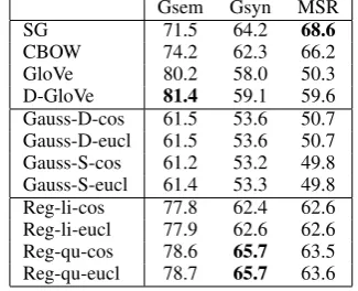
Table 1: Results for the analogy completion task (accuracy). Reg-li-* and Reg-qu-* are our models with a linear and quadratic kernel.
Gsem Gsyn MSR
SG 71.5 64.2 68.6
CBOW 74.2 62.3 66.2
GloVe 80.2 58.0 50.3
D-GloVe 81.4 59.1 59.6 Gauss-D-cos 61.5 53.6 50.7 Gauss-D-eucl 61.5 53.6 50.7 Gauss-S-cos 61.2 53.2 49.8 Gauss-S-eucl 61.4 53.3 49.8 Reg-li-cos 77.8 62.4 62.6 Reg-li-eucl 77.9 62.6 62.6 Reg-qu-cos 78.6 65.7 63.5 Reg-qu-eucl 78.7 65.7 63.6
Reg-li-eucl word vectors, obtained using linear kernel, compared using Euclidean distance; Reg-qu-cos word vectors, obtained using
quadratic kernel, compared using cosine similarity;
Reg-qu-eucl word vectors, obtained using quadratic kernel, compared using Euclidean distance;
Reg-li-prod Gaussian word regions, obtained us-ing linear kernel, compared usus-ing the inner productE;
Reg-li-wprod Gaussian word regions estimated using the weighted variant, obtained using linear kernel, compared using the inner prod-uctE;
Reg-li-JS Gaussian word regions, obtained us-ing linear kernel, compared usus-ing the Jensen-Shannon divergence;
Reg-li-wJS Gaussian word regions estimated us-ing the weighted variant, obtained usus-ing lin-ear kernel, compared using Jensen-Shannon divergence.
4.1 Analogy Completion
Analogy completion is a standard evaluation task for word embeddings. Given a pair(w1, w2) and
a word w3 the goal is to find the word w4 such
thatw3 andw4are related in the same way asw1
andw2. To solve this task, we predict the wordw4
which is most similar tow2−w1 +w3, either in
Test Set7 and the Microsoft Research Syntactic
Analogies Dataset8. The former contains both
se-mantic and syntactic relations, for which we show the results separately, respectively referred to as Gsem and Gsyn; the latter only contains syntactic relations and will be referred to as MSR. The re-sults are shown in Table1. Recall that the param-eters of D-GloVe were tuned on the Google Anal-ogy Test Set, hence the results reported for this model for Gsem and Gsyn might be slightly higher than what would normally be obtained. Note that for our model, we can only use word vectors for this task.
We outperform SG and CBOW for Gsem and Gsyn but not for MSR, and we outperform GloVe and D-GloVe for Gsyn and MSR but not for Gsem. The vectors from the Gaussian embedding model are not competitive for this task. For our model, using Euclidean distance slightly outperforms us-ing cosine. For GloVe, SG and CBOW, we only show results for cosine, as this led to the best re-sults. For D-GloVe, we used the likelihood-based similarity measure proposed in the original paper, which was found to outperform both cosine and Euclidean distance for that model.
For our model, the quadratic kernel leads to bet-ter results than the linear kernel, which is some-what surprising since this task evaluates a kind of linear regularity. This suggests that the ad-ditional flexibility that results from the quadratic kernel leads to more faithful context word repre-sentations, which in turn improves the quality of the target word vectors.
4.2 Similarity Estimation
To evaluate our model’s ability to measure sim-ilarity we use 12 standard evaluation sets9, for
which we will use the following abbreviations: S1: MTurk-287, S2:RG-65, S3:MC-30, S4:WS-353-REL, S5:WS-353-ALL, S6:RW-STANFORD, S7: YP-130, S8:SIMLEX-999, S9:VERB-143, S10: WS-353-SIM, S11:MTurk-771, S12:MEN-TR-3K. Each of these datasets contains similarity judgements for a number of word pairs. The task evaluates to what extent the similarity scores pro-duced by a given word embedding model lead to
7https://nlp.stanford.edu/projects/ glove/
8http://research.microsoft.com/en-us/
um/people/gzweig/Pubs/myz_naacl13_test_ set.tgz
9https://github.com/mfaruqui/ eval-word-vectors
the same ordering of the word pairs as the pro-vided ground truth judgments. The evaluation metric is the Spearmanρ rank correlation coeffi-cient. For this task, we can either use word vectors or word regions. The results are shown in Table2. For our model, the best results are obtained when using word vectors and the Euclidean dis-tance (Reg-qu-eucl), although the differences with the word regions (Reg-qu-wprod) are small. We useprod to refer to the configuration where simi-larity is estimated using the inner product, whereas we write JS for the configurations that use Jensen-Shannon divergence. Moreover, we usewprodand wJS to refer to the weighted variant for estimating the Gaussians. We can again observe that using a quadratic kernel leads to better results than us-ing a linear kernel. As the weighted versions for estimating the Gaussians do not lead to a clear im-provement, for the remainder of this paper we will only consider the unweighted variant.
With the exception of S9, our model substan-tially outperforms the Gaussian word embedding model. Of the standard models SG and D-GloVe obtain the strongest performance. Compared to our model, these baseline models achieve similar results for S2, S10, S11 and S12, worse results for S1, S3, S4, S5, S6 and better results for S7, S8 and S9. Two general trends can be observed. First, the data sets where our model performs better tend to be datasets which describe semantic relatedness rather than pure synonymy. Second, the standard models appear to perform better on data sets that contain verbs and adjectives, as opposed to nouns.
4.3 Modeling properties
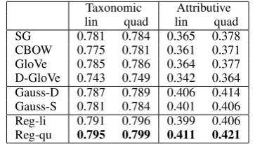
In (Rubinstein et al., 2015), it was analysed to what extent word embeddings can be used to iden-tify concepts that satisfy a given attribute. While good results were obtained for taxonomic prop-erties, attributive properties such as ‘dangerous’, ‘round’, or ‘blue’ proved to be considerably more problematic. We may expect region-based mod-els to perform well on this task, since each of these attributes then explicitly corresponds to a re-gion in space. To test this hypothesis, Table 3
shows the results for the same 7 taxonomic prop-erties and 13 attributive propprop-erties as in ( Rubin-stein et al., 2015), where the positive and nega-tive examples for all 20 properties are obtained from the McRae feature norms data (McRae et al.,
Table 2: Results for similarity estimation (Spearmanρ). Reg-li-* and Reg-qu-* are our models with a linear and quadratic kernel.
S1 S2 S3 S4 S5 S6 S7 S8 S9 S10 S11 S12
SG 0.656 0.773 0.789 0.648 0.709 0.459 0.500 0.415 0.435 0.773 0.655 0.731 CBOW 0.644 0.768 0.740 0.532 0.622 0.419 0.341 0.361 0.343 0.707 0.597 0.693 GloVe 0.595 0.755 0.746 0.515 0.577 0.318 0.533 0.382 0.354 0.690 0.652 0.724 D-GloVe 0.659 0.788 0.785 0.555 0.651 0.401 0.535 0.413 0.388 0.778 0.656 0.746
Gauss-D-cos 0.591 0.622 0.661 0.403 0.501 0.249 0.388 0.337 0.411 0.640 0.599 0.643 Gauss-D-eucl 0.591 0.623 0.661 0.403 0.501 0.250 0.388 0.338 0.411 0.641 0.599 0.643 Gauss-D-prod 0.588 0.618 0.658 0.399 0.498 0.213 0.356 0.326 0.409 0.631 0.588 0.633 Gauss-D-JS 0.598 0.619 0.665 0.403 0.532 0.288 0.381 0.339 0.410 0.643 0.599 0.644 Gauss-S-cos 0.593 0.632 0.681 0.409 0.506 0.256 0.392 0.337 0.416 0.649 0.601 0.644 Gauss-S-eucl 0.593 0.632 0.681 0.409 0.507 0.356 0.393 0.337 0.416 0.649 0.603 0.644 Gauss-S-prod 0.591 0.619 0.659 0.403 0.505 0.312 0.389 0.328 0.412 0.633 0.591 0.633 Gauss-S-JS 0.598 0.622 0.667 0.405 0.533 0.288 0.385 0.349 0.410 0.643 0.601 0.644 Reg-li-cos 0.666 0.764 0.821 0.652 0.713 0.489 0.469 0.354 0.361 0.734 0.642 0.739 Reg-li-eucl 0.668 0.766 0.821 0.654 0.715 0.489 0.469 0.359 0.361 0.734 0.643 0.739 Reg-li-prod 0.661 0.759 0.818 0.634 0.710 0.481 0.445 0.358 0.360 0.724 0.641 0.729 Reg-li-wprod 0.663 0.761 0.819 0.638 0.711 0.482 0.446 0.359 0.361 0.725 0.642 0.731 Reg-li-JS 0.663 0.758 0.815 0.638 0.709 0.479 0.443 0.359 0.361 0.723 0.641 0.729 Reg-li-wJS 0.665 0.760 0.816 0.638 0.710 0.481 0.445 0.359 0.361 0.725 0.641 0.731 Reg-qu-cos 0.684 0.781 0.839 0.662 0.723 0.505 0.479 0.367 0.368 0.777 0.656 0.744 Reg-qu-eucl 0.685 0.781 0.839 0.664 0.723 0.509 0.479 0.367 0.368 0.779 0.656 0.744 Reg-qu-prod 0.681 0.780 0.831 0.658 0.719 0.501 0.478 0.355 0.331 0.778 0.653 0.741 Reg-qu-wprod 0.684 0.788 0.831 0.663 0.721 0.501 0.475 0.370 0.365 0.778 0.653 0.739 Reg-qu-JS 0.680 0.781 0.826 0.661 0.715 0.497 0.471 0.328 0.355 0.771 0.649 0.721 Reg-qu-wJS 0.678 0.782 0.824 0.662 0.712 0.498 0.469 0.326 0.351 0.771 0.644 0.720
Table 3: Results for McRae feature norms (F1). Reg-li and Reg-qu are our models with a linear and quadratic kernel.
Taxonomic Attributive lin quad lin quad SG 0.781 0.784 0.365 0.378 CBOW 0.775 0.781 0.361 0.371 GloVe 0.785 0.786 0.364 0.377 D-GloVe 0.743 0.749 0.342 0.364 Gauss-D 0.787 0.789 0.406 0.414 Gauss-S 0.781 0.784 0.401 0.406 Reg-li 0.791 0.796 0.399 0.406 Reg-qu 0.795 0.799 0.411 0.421
5-fold cross-validation to train a binary SVM for each property and compute the average F-score due to unbalanced class label distribution. We separately present results for SVMs with a linear and a quadratic kernel. The results indeed support the hypothesis that region-based models are well-suited for this task, as both the Gaussian embed-ding model and our model outperform the standard word embedding models.
4.4 Hypernym Detection
For hypernym detection, we have used the follow-ing 5 benchmark data sets10: H1 (Baroni et al., 2012), H2 (Baroni and Lenci,2011), H3 (
Kotler-10https://github.com/stephenroller/ emnlp2016
man et al., 2010), H4 (Levy et al.,2014) and H5 (Turney and Mohammad,2015). Each of the data sets contains positive and negative examples, i.e. word pairs that are in a hypernym relation and word pairs that are not. Rather than treating this problem as a classification task, which would re-quire selecting a threshold in addition to producing a score, we treat it as a ranking problem. In other words, we evaluate to what extent the word pairs that are in a valid hypernym relation are the ones that receive the highest scores. We use average precision as our evaluation metric.
Apart from our model, the Gaussian embedding model is the only word embedding model that can by design support unsupervised hyperynym detec-tion. As an additional baseline, however, we also show how Skip-gram performs when using cosine similarity. While such a symmetric measure can-not faithfully model hypernyny, it was nonetheless found to be a strong baseline for hypernymy mod-els (Vuli´c et al., 2016), due to the inherent diffi-culty of the task. We also compare with a num-ber of standard bag-of-words based models for de-tecting hypernyms: WeedsPrec (Kotlerman et al.,
2010), ClarkeDE (Clarke,2009) and invCL (Lenci and Benotto, 2012). These latter models take as input the PPMI weighted co-occurrence counts.
[image:8.595.90.272.415.518.2]Table 4: Results for hypernym detection (AP). Reg-li-* and Reg-qu-* are our models with a lin-ear and quadratic kernel.
Model H1 H2 H3 H4 H5
WeedsPrec 0.565 0.376 0.611 0.414 0.685 ClarkeDE 0.588 0.397 0.621 0.426 0.699 invCL 0.603 0.416 0.693 0.439 0.756 SG 0.682 0.434 0.712 0.455 0.789 Gauss-D-KL 0.865 0.505 0.806 0.515 0.815 Gauss-S-KL 0.823 0.498 0.801 0.507 0.789 Gauss-D-Cos 0.846 0.499 0.801 0.509 0.811 Gauss-S-Cos 0.813 0.484 0.799 0.501 0.778 Gauss-D-KLC 0.868 0.511 0.809 0.519 0.815 Gauss-S-KLC 0.835 0.501 0.804 0.511 0.795 Reg-li-KL 0.867 0.501 0.805 0.505 0.801 Reg-qu-KL 0.871 0.512 0.811 0.521 0.814 Reg-li-Cos 0.871 0.502 0.807 0.508 0.804 Reg-qu-Cos 0.873 0.513 0.818 0.525 0.819 Reg-li-KLC 0.874 0.509 0.812 0.511 0.806 Reg-qu-KLC 0.878 0.519 0.825 0.531 0.823
in which Kullback-Leibler divergence is used to compare word regions. Surprisingly, both for our model and for the Gaussian embedding model, we find that using cosine similarity between the word vectors outperforms using the word regions with KL-divergence. In general, our model out-performs the Gaussian embedding model and the other baselines. Given the effectiveness of the co-sine similarity, we have also experimented with the following metric:
hyp(w1, w2) = (1−cos(w1, w2))·KL(fw1||fw2)
The results are referred to as li-KLC and Reg-qu-KLC in Table4. These results suggest that the word regions can indeed be useful for detecting hypernymy, when used in combination with cosine similarity. Intuitively, forw2to be a hypernym of
w1, both words need to be similar and w2 needs
to be more general thanw1. While word regions
are not needed for measuring similarity, they seem essential for modeling generality (in an unsuper-vised setting).
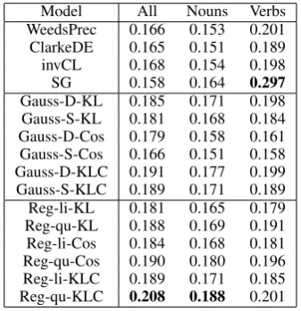
[image:9.595.332.501.109.284.2]The datasets considered so far all treat hyper-nyms as a binary notion. In (Vuli´c et al., 2016) a evaluation set was introduced which contains graded hypernym pairs. The underlying intuition is that e.g. cat and dog are more typical/natural hy-ponyms of animal than dinosaur or amoeba. The results for this data set are shown in Table 5. In this case, we use Spearmanρas an evaluation met-ric, measuring how well the rankings induced by different models correlate with the ground truth. Following (Vuli´c et al.,2016), we separately men-tion results for nouns and verbs. In the case of
Table 5: Results for HyperLex (Spearmanρ). Reg-li-* and Reg-qu-* are our models with a linear and quadratic kernel.
Model All Nouns Verbs WeedsPrec 0.166 0.153 0.201 ClarkeDE 0.165 0.151 0.189 invCL 0.168 0.154 0.198 SG 0.158 0.164 0.297
Gauss-D-KL 0.185 0.171 0.198 Gauss-S-KL 0.181 0.168 0.184 Gauss-D-Cos 0.179 0.158 0.161 Gauss-S-Cos 0.166 0.151 0.158 Gauss-D-KLC 0.191 0.177 0.199 Gauss-S-KLC 0.189 0.171 0.189 Reg-li-KL 0.181 0.165 0.179 Reg-qu-KL 0.188 0.169 0.191 Reg-li-Cos 0.184 0.168 0.181 Reg-qu-Cos 0.190 0.180 0.196 Reg-li-KLC 0.189 0.171 0.185 Reg-qu-KLC 0.208 0.188 0.201
nouns, our findings here are broadly in agreement with those from Table4 Interesting, for verbs we find that Skip-gram substantially outperforms the region based models, which is in accordance with our findings in the word similarity experiments.
5 Conclusions
We have proposed a new word embedding model, which is based on ordinal regression. The input to our model consists of a number of rankings, cap-turing how strongly each word is related to each context word in a purely ordinal way. Word vec-tors are then obtained by embedding these rank-ings in a low-dimensional vector space. Despite the fact that all quantitative information is disre-garded by our model (except for constructing the rankings), it is competitive with standard methods such as Skip-gram, and in fact outperforms them in several tasks. An important advantage of our model is that it can be used to learn region repre-sentations for words, by using a quadratic kernel. Our experimental results suggest that these regions can be useful for modeling hypernymy.
Acknowledgments
References
Marco Baroni, Raffaella Bernardi, Ngoc-Quynh Do, and Chung-chieh Shan. 2012. Entailment above the word level in distributional semantics. In Proceed-ings of the 13th Conference of the European Chap-ter of the Association for Computational Linguistics. pages 23–32.
Marco Baroni and Alessandro Lenci. 2011. How we blessed distributional semantic evaluation. In Pro-ceedings of the GEMS 2011 Workshop on GEomet-rical Models of Natural Language Semantics. Asso-ciation for Computational Linguistics, pages 1–10. Wei Chu and S Sathiya Keerthi. 2005. New approaches
to support vector ordinal regression. InICML. pages 145–152.
Daoud Clarke. 2009. Context-theoretic semantics for natural language: an overview. In Proceedings of the Workshop on Geometrical Models of Natural Language Semantics. pages 112–119.
Katrin Erk. 2009. Representing words as regions in vector space. InProceedings of the Thirteenth Con-ference on Computational Natural Language Learn-ing. pages 57–65.
Manaal Faruqui and Chris Dyer. 2014. Improving vec-tor space word representations using multilingual correlation. InProceedings of the 14th Conference of the European Chapter of the Association for Com-putational Linguistics. pages 462–471.
Andrea Frome, Gregory S. Corrado, Jonathon Shlens, Samy Bengio, Jeffrey Dean, Marc’Aurelio Ranzato, and Tomas Mikolov. 2013. Devise: A deep visual-semantic embedding model. InProc. NIPS. pages 2121–2129.
Yoav Goldberg. 2016. A primer on neural network models for natural language processing. Journal of Artificial Intelligence Research57:345–420. Yoav Goldberg and Omer Levy. 2014. word2vec
explained: Deriving mikolov et al.’s negative-sampling word-embedding method. arXiv preprint arXiv:1402.3722.
Abhijeet Gupta, Gemma Boleda, Marco Baroni, and Sebastian Pad´o. 2015. Distributional vectors encode referential attributes. InProc. EMNLP. pages 12– 21.
Shoaib Jameel and Steven Schockaert. 2016. D-glove: A feasible least squares model for estimating word embedding densities. InProceedings of the 26th In-ternational Conference on Computational Linguis-tics. pages 1849–1860.
Joo-Kyung Kim and Marie-Catherine de Marneffe. 2013. Deriving adjectival scales from continuous space word representations. InProc. EMNLP. pages 1625–1630.
Lili Kotlerman, Ido Dagan, Idan Szpektor, and Maayan Zhitomirsky-Geffet. 2010. Directional distribu-tional similarity for lexical inference. Natural Lan-guage Engineering16:359–389.
Alessandro Lenci and Giulia Benotto. 2012. Identify-ing hypernyms in distributional semantic spaces. In
Proceedings of *SEM. pages 75–79.
Omer Levy, Yoav Goldberg, and Israel Ramat-Gan. 2014. Linguistic regularities in sparse and explicit word representations. InProc. CoNLL. pages 171– 180.
Tie-Yan Liu. 2009. Learning to rank for information retrieval. Foundations and Trends in Information Retrieval3:225–331.
Ken McRae, George S Cree, Mark S Seidenberg, and Chris McNorgan. 2005. Semantic feature produc-tion norms for a large set of living and nonliving things. Behavior Research Methods37:547–559. Tomas Mikolov, Kai Chen, Greg Corrado, and Jeffrey
Dean. 2013a. Efficient estimation of word represen-tations in vector space. InInternational Conference on Learning Representations.
Tomas Mikolov, Ilya Sutskever, Kai Chen, Gregory S. Corrado, and Jeffrey Dean. 2013b. Distributed rep-resentations of words and phrases and their compo-sitionality. InProceedings of the 27th Annual Con-ference on Neural Information Processing Systems. pages 3111–3119.
Neha Nayak. 2015. In learning hyperonyms over word embeddings. Technical report, Student technical re-port.
Jeffrey Pennington, Richard Socher, and Christo-pher D. Manning. 2014. Glove: Global vectors for word representation. InProc. EMNLP. pages 1532– 1543.
Sascha Rothe and Hinrich Sch¨utze. 2016. Word embedding calculus in meaningful ultradense sub-spaces. In Proceedings of the 54th Annual Meet-ing of the Association for Computational LMeet-inguis- Linguis-tics. pages 512–517.
Dana Rubinstein, Effi Levi, Roy Schwartz, and Ari Rappoport. 2015. How well do distributional mod-els capture different types of semantic knowledge? In Proceedings of the 53rd Annual Meeting of the Association for Computational Linguistics. pages 726–730.
Steven Schockaert and Jae Hee Lee. 2015. Qualita-tive reasoning about directions in semantic spaces. InProceedings of the International Joint Conference on Artificial Intelligence. pages 3207–3213. Amnon Shashua and Anat Levin. 2002. Ranking with
P. D. Turney and P. Pantel. 2010. From frequency to meaning: Vector space models of semantics. Jour-nal of Artificial Intelligence Research37:141–188. Peter D Turney and Saif M Mohammad. 2015.
Ex-periments with three approaches to recognizing lex-ical entailment. Natural Language Engineering
21(03):437–476.
Ivan Vendrov, Ryan Kiros, Sanja Fidler, and Raquel Urtasun. 2016. Order-embeddings of images and language. InInternational Conference on Learning Representations.
Luke Vilnis and Andrew McCallum. 2015. Word rep-resentations via gaussian embedding. In Proceed-ings of the International Conference on Learning Representations.
Ivan Vuli´c, Daniela Gerz, Douwe Kiela, Felix Hill, and Anna Korhonen. 2016. Hyperlex: A large-scale evaluation of graded lexical entailment. arXiv. Will Y Zou, Richard Socher, Daniel M Cer, and
Christopher D Manning. 2013. Bilingual word em-beddings for phrase-based machine translation. In