Abstract—In this paper, a special class of trajectory optimization problems is formulized and solved. It involves the optimization of different Unmanned Vehicle (UMV) trajectories, which are coupled through reciprocal constraints. It is shown in the paper that searching for a solution to the problem at hand may stipulate not just planning a longer than the shortest possible path for each UMV, but also choosing slower travel speeds in order to coordinate between the UMVs. Although it seems that solving the problem possesses merits, it has been only partially treated before. Here we suggest solving it by utilizing an evolutionary approach which involves a new algorithmic feature that allows striving towards the desired optimality. The approach is demonstrated and studied through solving and simulating several trajectory planning problems. It is shown that a wide range of problems might be related to that class of problems.
Index Terms—Trajectory planning, unmanned vehicles,
evolutionary algorithms
I. INTRODUCTION
MVs have been a major research field in the last two decades. The design, control, and planning of their tasks have been widely investigated [1,7,9-12,15]. Planning trajectories for several UMVs is significantly more difficult than the path planning problem for single robot systems since the size of the joint state space of the robot increases exponentially to the number of robots [2]. The motivation for cooperation between UMVs/robots has been based on the recognition that there are several tasks that can be performed more efficiently and robustly using multiple robots [3,8,14]. Another problem treating the interaction between UMVs deals with planning of paths for different UMVs with emphasize on avoiding collisions between them [2], where often the individual paths are also optimized [13].
The current paper deals with a wider definition for the coupled trajectories problem. Here the task of the UMVs is not mutual with each UMV having its own task and therefore its own related optimization problem, possibly performing in totally different workspaces. Nevertheless, these individual optimization problems are coupled through Manuscript received November 30, 2010; revised December 27, 2011. (This work was supported by ORT Braude research grant no. 5000.838.1.2.11.
Gideon Avigad is a Senior lecturer in the Mechanical Engineering Department, Braude College of Engineering, POB 78, Karmiel 21982, Israel e-mail: [email protected]).
Erella Eisenstadt is a Lecturer in the Mechanical Engineering Department, Braude College of Engineering, POB 78, Karmiel 21982, Israel (e-mail: [email protected]).
Miri Weiss-Cohen is a Senior lecturer in the Software Engineering Department of Braude College of Engineering, POB 78, Karmiel 21982, Israel (e-mail: miri@ braude.ac.il).
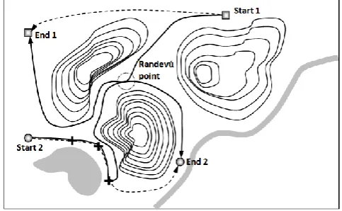
reciprocal constraints. For example, depict the map in Fig. 1. Suppose that an UMV has to travel from point “start 1” to the point designated as “end 1”. The planners are asked to plan a path/trajectory for this aircraft while minimizing its travel time and avoiding mountains. The optimal solution for this task is designated in Fig. 1 by a dashed curve between these points. Now consider the same map, but this time considered by different planners. Their task is to plan the trajectory of an UMV traveling from “start 2” to “end 2” and having to deliver supplies to a set of pickup points designated by plusses while also avoiding the mountains. An optimal solution for this problem is designated by a dashed curve passing through these points. Depicting each of these problems per se, it is clear that the problems might be solved by totally different teams, possibly with different expertise and backgrounds. Yet, in the current study, these teams are forced to cooperate and take mutual decisions as a result of reciprocal constraints. An example for such a constraint is the need for the UMVs to have a rendezvous region that will serve as a refueling point. This demand constrains the designers to consider altering their plans in order to coordinate their trajectories, yet preserving the inspiration for optimization (shortest path). It is noted that both the location and schedule of the meeting should be found as part of the optimization problem solution. Moreover, the problem is not restricted to constraints between aerial or ground vehicles, with a combination of them being possible.
Fig. 1. A workspace (map) where two UMVs’ trajectories are to be optimized, while meeting reciprocal constraints.
The existing methods for solving the problem of different UMVs’ trajectories, which are optimized while avoiding collisions among them may be divided into two categories: a centralized approach, where the configuration spaces of the individual robots are combined into one composite configuration space which is then searched for a path for the whole composite system. In contrast, the decoupled approach first computes separate paths for the individual
Trajectory Planning for Multi UMVs with
Reciprocal Constraints
Gideon Avigad, Erella Eisenstadt, and Miri Weiss-Cohen
[image:1.595.309.551.509.658.2]robots and then resolves possible conflicts of the generated paths. Most of the attempts to share components between solutions to several problems that are coupled through constraints are associated with the design of a product family. A product family is a group of related products that share common components and/or subsystems – yet satisfy a variety of market niches [16].
A common trajectory optimization problem may be defined as follows:
Find a trajectory P(x,t) in order to minimize
(
P
)
subject to g x t( , )0 and h x t( , )0. Where x is a vector of position coordinates and t is the time. ( )P may be the path length, path time, change of direction within the path etc. The current problem is defined as follows:Find trajectories (a solution) ( , )P x t where 1
1
( , ) [ ( , ),..., K( K, )]T
P x t P x t P x t in order to: ( ( )),
Min P (1)
1
1 1
( )P [ (P x t( , ),.... i(P x ti( , ),...,i K(PK(xK, )]t T
subject to: gj( ( , ))P x t 0 for 1 j Jand h P x te( ( , ))0 for1 e E, where xi is the position coordinate of the i-th
trajectory of x and t is the time. i(P x ti( , )i is the objective of the i-th trajectory's planning, which may differ, from one trajectory to the other. gj( ( , ))P x t and h P x te( ( , ))are inequality and equality constraints, respectively. The dependence of the constraints functions (g and h) on several trajectories engender coupling between the trajectories.
It is noted that the definition as given in (1) is not a definition of a multi-objective problem. If a MOP is at hand, the vector xi would be unanimous to all objectives and not
distinct to each objective as is the case in the current problem. This is further highlighted by the different prime indices given to the path (i.e., i). In this case, the problem is formalized as a constrained single objective problem, where the objective function is a utility of all of the different problems' objective functions. The problem is defined as follows:
( ( )), Min P
1
( )
(
( , )
K
i i
i i
i
P
P x t
(2)Subject to:
g P x t
i( ( , ))
0
for1
i
K
,( ( , ))
0
j
r P x t
for1
j
J
, where gi is the i-thtrajectory specific constraints and rj is the j-th reciprocal
constraint.iis the i-th trajectory weight, which reflects the designers view concerning the importance of the trajectory with respect to the other trajectories. This weight may also include a scaralaizing element. In the current paper, we utilize just for scaralizing as we regard all problems to be important to the same extent. It is noted that the definition in (2) is a weighted sum approach.
II. REVOLUTE PRISMATIC CHAIN (RPC) ALGORITHM Genetic Algorithms (GAs) are considered to be a part of Evolutionary Computation (EC) methods. They are used extensively for solving single objective problems and are also an appealing option when Multi Objective Optimization
Problems (MOPs) are to be solved [4-6, 17].
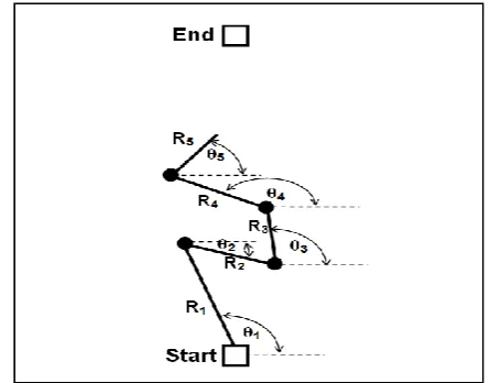
[image:2.595.314.537.283.457.2]In this work, a new approach is suggested, which is termed the Revolute Prismatic Chain (RPC). The RPC algorithm combines gradually extracting (prismatic) and tilting (revolute) parameters using Genetic Algorithms' evolutionary parameters. The RPC is constructed from a predefined number of sections. A section represents the length of travel made by the UMV at each time step. Each section is anchored at the end of the prior section (the first section is anchored to the starting point). The angle at which each section is extended is coded as a parameter. Also coded is the length of each section. This means that the speed of travel is coded by this length (length per time is the speed of travel). The maximal length is the maximal speed that may be obtained by the UMV. Note that the speed at each section is the mean velocity at this section. Fig. 2 depicts a five section RPC. It is noted that the end of the RPC is not encored to the end point and is located wherever the last section ends.
Fig. 2. The RPC with 5 sections. The length of each section and its angle with respect to the previous section are coded with the evolutionary algorithm code.
We utilized an elite based EA in order to search for the solutions to problem [7]. An individual within the population is constructed out of several chromosomes, each coding one trajectory out of the coupled problems' trajectories. Therefore, a decoded individual is a complete solution to the problem (whether successful or not).
The coded parameters are decoded to intervals such that N
i all for Ri o i o
,... 1 1
0 ; 180
180
. The
number of the RPC sections, N, and the number of members in a set (number of RPC's) is K, are predefined. Also predefined are the population size n and the number of generations G. The influence of the constraints violations on the evolution has been introduced to the algorithm through a procedure detailed in the following code. The evolutionary algorithm is an elite based GA[7], described by the following pseudo code:
The GA pseudo code
a. Initialize a population
P
t with n individuals. Also, create a population Qt = Ptb. While tG
d. For each individual x in Rtcompute: (x), d(x),
(x) as detailed in calculations I, II, III, respectively.
e. Create Elite population Pt+1 of size n from Rt
(procedure I )
f. Create offspring population Qt1*of size n from Rt by Tournament selection (procedure II )
g. Perform Crossover to obtain Qt1** from * 1 t Q . h. Perform Mutation' to obtain Qt1 fromQt1**. i. Set t t 1 and go to b.
Calculation I: Φ(x)
1. Find trajectories:
2. 1
1
( , ) [ ( , ),..., K( K, )]T
P x t P x t P x t 3. Find
1
1 1
( ( , ))P x t [ (P x t( , ),.... i(P x ti( , ),...,i K(PK(xK, )]t T
and compute
1
( ) ( ( , )
K
i i
i i
i
x
P x t
Calculation II: d(x)
1. Find the distance from the i-th RPC end point, to the i-th end point as follows:
2.
1
[image:3.595.53.523.524.743.2]1
( , ) | ( , ) 0
max ( , )
( )
( , ) | ( , ) 0
max ( , )
i i i i
end i final
i K
i i i i
end i
i K g x t g x t
Then x P x t
d x
g x t g x t
Then x P x t
The distance is in fact the longest distance of an RPC end point to its target point. If an RPC bumps into an obstacle, than this bumping point, is regarded as the end of the RPC.
Calculation III: δ(x)
1. For all trajectories of x compute
, ( , ) ( , ) 1,...., ;
i l
i l P x ti P x tl for all i K i l
Compute ( )x (i l, ) where , is a problem related function.
Note: In all examples
( ( , )) ( , )
i
i i
P x t Length of thetrajectory P x t
,
1 1,...,
i for all i K
. In the first example where the reciprocal constraint is to keep the distance between trajectories smaller than dmin, ( )x (i l,), in all other examples, where the reciprocal constraint is to achieve ameeting point, ,
, ( ) min( i l)
i l x
.
III. EXAMPLES
In this section, several examples are solved. The examples include problems with two and three coupled trajectory optimization problems. In all examples, 50% crossover with Gaussian distributed mutation with probability of 5% has been utilized.
A. Example 1
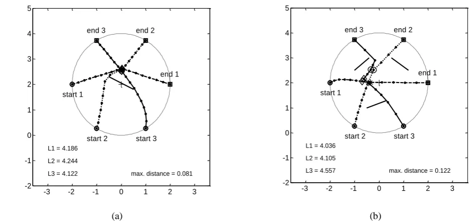
Here two similar cases are considered. In both of them, three UMVs’ trajectories are optimized in order to find the shortest path for each while avoiding obstacles. The reciprocal constraint is that each UMV has to meet all other UMVs once during the travel. The difference between the two cases of this example is that, in the first, there is just one obstacle, while in the second, there are three obstacles. The optimal solutions for the two cases are shown in Fig. 3a and 3b, respectively.
(a) (b)
Fig. 3. Three UMVs’ optimal trajectories with a constraint they must all rendezvous somewhere sometime as they travel. One obstacle (3a) and three obstacles (3b).
-3 -2 -1 0 1 2 3 -2
-1 0 1 2 3 4 5
end 1 end 2 end 3
start 1
start 2 start 3
L1 = 4.186
L2 = 4.244
L3 = 4.122 max. distance = 0.081
-3 -2 -1 0 1 2 3 -2
-1 0 1 2 3 4 5
end 1 end 2 end 3
start 1
start 2 start 3
L1 = 4.036
L2 = 4.105
B. Example 2
In this example, two UMVs move from different starting points to different end points while traveling the shortest path and avoiding a big obstacle (in Fig. 4, its boundaries are bold lines), yet are bound to meet once, possibly for the purpose of refueling. The place and time of the meeting is not specified. The minimal distance at the time of meeting is set to dmin<0.1. In terms of (1), the
problem may be defined as follows: T
2 1,L ] L [
1
( , ) ( , ) ( , ) :
( , ) ( , ) 0
i i
i i
i
i j
P x t P x t j J P x t
P x t O x t
(obstacle avoidance)
* * *
* *
2
, ( , ), ( , ) ( , ) :
( , ) ( , ) 0
i j
i j
i j
i j
t P x t P x t P x t
P x t P x t
(meeting point at least at one t*) C. Example 3
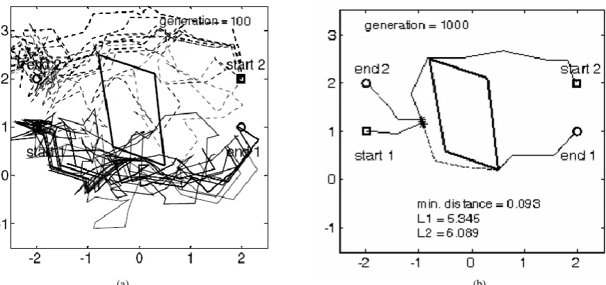
The purpose of the second example is to show the applicability of the suggested algorithm to solve multi trajectory planning problems for which, apart from optimizing the trajectories, avoidance of collisions is important. Instead of a constraint to keep the distance between the UMVs, less than a predefined distance, here, the constraint is altered such that, the distance between the UMVs should not be less than the predefined distance. It is further noted that the UMVs are bound to travel in opposite directions due to the location of their related starting and end points. 20-section RPC coded solutions, where each section may vary between 0.0 and 0.8, were run for 1000 generations
The populations after 100 and 1000 (final) generations are depicted in Fig. 4a and 4b, respectively. It is observed that after 100 generations not all RPCs reach the end point, with a few of them bumping into the obstacle. At the end of the run (after 1000 generations), the solutions converge to a single solution, which is depicted in Fig. 4b. Note that for the meeting to take place, one UMV (the one that started on the left) had to wait for the other to come around the obstacle and then continue to travel to its end point within the speed limit (determined by the boundaries set to the length of the RPC sections). This means that the other UMV had to travel fast at the beginning and then slow down after the rendezvous.
Fig. 5 (a)-(b) depicts a three-UMV trajectory planning problem. Fig. 5a depicts four trajectory sections evolved by using the paper’s approach. The dashed lines show the minimal distance between the UMVs during their travel. The trajectories are almost straight lines and the distance is within the allowed limit. Fig. 5b depicts the same problem; this time the trajectories are being evolved by using RPCs with 20 sections. It is clear that non-violation of the constraint is more ensured, yet at the cost of computational time and optimality.
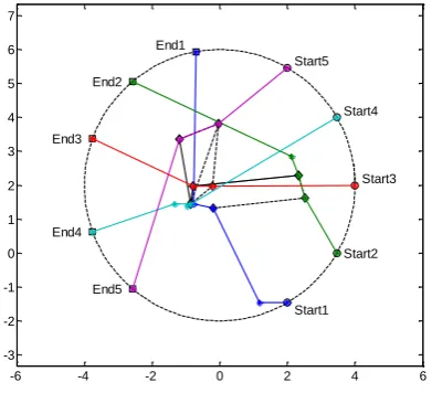
Fig. 6 depicts the evolved trajectories of the five-UMV problem (RPC are with five sections each).
IV. SUMMARY AND CONCLUSIONS
In the paper, a formulation for a class of problems has been suggested. A problem belonging to this class involves the optimization of UMV trajectories that are subject to reciprocal constraints. The definition incorporates a wide range of problems, including cases where the UMVs do not share the same workspace. Reciprocal constraints between trajectories may be associated with demands such as the following:
[image:4.595.81.517.502.706.2]
(a) (b)
(a) (b) Fig. 5: (a) Three UMVs’ trajectories with 3-section RPCs.( b) Three UMVs’ trajectories with 5-section RPCs.
Fig. 6. Five UMVs’ trajectories with 5 section RPCs
(a) At any time, keep the distance between the UMVs below a predefined distance; (b) At any time, keep the distance between the UMVs above a predefined distance (avoiding collisions); (c). Always allow line of sight contact between the UMVs; (d). Always occupy one UMV at each sub-workspace, etc.
A robust approach has been suggested that can cope with solving all of these problems. It involves the representation of a path by a telescopic antenna. The length and orientation of the antenna’s sections are evolved by a genetic algorithm.
REFERENCES
[1] G. Avigad, and K. Deb, “The sequential optimization-constraint multi-objective problem and its applications for robust planning of robot paths,” in Proc. IEEE Congress on Evolutionary
Computation (CEC'2007), September 2007, pp. 2101–2108.
[2] M. Bennewitz, W. Burgard, and S. Thrun, “Optimizing schedules for prioritized path planning of multi-robot systems,” in Proc. 2001 ICRA. IEEE International Conference on Robotics and
Automation, 2001, pp. 1271–1276.
[3] W. Burgard, M. Moors, D. Fox, R. Simmons, and S. Thrun, “Collaborative multi-robot exploration,” in Proc. IEEE Int. Conf. on Robotics and Automation, San Francisco, CA, 2000, pp. 476– 481.
[4] O. Castillo, L. Trujillo, and P. Melin, “Multiple objective genetic algorithms for path-planning optimization in autonomous mobile robots,” Soft Computing, vol. 11, pp. 269–279, 2007.
[5] Z. Cai, and Z. Peng, “Cooperative coevolutionary adaptive genetic algorithm in path planning of cooperative multi-mobile robot aystems,” J. of Intelligent and Robotic Systems, vol. 33(1), pp. 61– 71, 2002.
[6] L. Chi-Ming, “Multicriteria–multistage planning for the optimal path selection using hybrid genetic algorithms,” Applied
Mathematics and Computation, vol. 180, pp. 549–558, 2006.
[7] K. Deb, A. Pratap, S. Agarwal, and T. A. Meyarivan, T. A, “Fast and elitist multi objective genetic algorithm: NSGA–II,” IEEE
Transactions on Evolutionary Computation, vol. 6(2), pp. 182–
197, 2002.
[8] B. Donald, L. Gariepy, and D. Rus, D., “Distributed manipulatio n of multiple objects using ropes,” in Proc. IEEE Int. Conf. on
Robotics and Automation, 2000, pp. 450–457.
[9] J. S. Jennings, G. Whelan, and W. F. Evans,. “Cooperative search and rescue with a team of mobile robots,” in Proc. IEEE Int. Conf.
on Advanced Robotics (ICAR), Monterey, CA. 1997, pp. 193–200.
[10] I. Kaminer, O. Yakimenko, A. Pascoal, and R. Ghabcheloo, (). “Path generation, path following and coordinated control for time-critical missions of multiple UAVs,” in Proc. American Control
Conf., Minneapolis, MN, 2006.
[11] M. Hebert, Intelligent unmanned ground vehicles: Autonomous
navigation research at Carnegie Mellon. Norwell, MA: Kluwer
Academic Publishers, 1997
[12] A. Moshaiov, G. Avigad, and N. Brauner, “Multi-objective path planning by the concept-based IEC method,” in Proc. 2004 IEEE
Int. Conference on Computational Cybernetics, ICCC 2004.
Vienna, Austria, 2004.
[13] S. Mittal, and K. Deb, “Three-dimensional path planning for UAVs using multi-objective evolutionary algorithms,” Proc.
Congress on Evolutionary Computation (CEC-2007), September,
2007, pp. 25–28.
[14] L. E. Parker, “Multiple mobile robot systems,” in Springer Handbook of Robotics, ch. 40, B. Siciliano and O. Khatib, Ed.. Springer, 2008.
[15] T. Sugar, and V. Kumar, “Control and coordination of multiple mobile robots in manipulation and material handling tasks,” in Experimental Robotics VI: Lecture Notes in Control and Information Sciences, vol. 250P. Corke, and J. Trevelyan, Eds.: Berlin: Springer-Verlag, 2000, pp. 15–24.
[16] T.W. Simpson, “Product platform design and optimization: status and promise,” in Proc. Design Eng. Technical Conf. and
Computers and Information in Eng. Conf. (DETC’03 ASME 2003),
Chicago, IL, 2003.
[17] R. Saravanan, S. Ramabalan, and C. Balamurugan, C., “Evolutionary multi-criteria trajectory modeling of industrial robots in the presence of obstacles,” Engineering Applications of Artificial Intelligence, vol. 22, pp. 329–342, 2009.
-6 -4 -2 0 2 4 6
-3 -2 -1 0 1 2 3 4 5 6 7
Start1 End1
Start2 End2
Start3 End3
Start4
End4
Start5
[image:5.595.70.266.306.484.2]