Abstract—In this paper, the descriptions on the development of a flow solver for the three-dimensional compressible Euler equations are presented. The underlying numerical scheme for the solver was based on the collisional Boltzmann model that produces the gas-kinetic BGK (Bhatnagaar-Gross-Krook) scheme. In constructing the desired algorithm, the convection flux terms were discretized by a semi-discrete finite difference method. The resulting inviscid flux functions were approximated by the gas-kinetic BGK scheme. To achieve higher order spatial accuracy, the cell interface primitive flow variables were reconstructed via the MUSCL (Monotone Upstream-Centered Schemes for Conservation Laws) interpolation method coupled with a min-mod limiter. As for advancing the solutions to another time level, an explicit-type time integration method known as the modified fourth-order Runge-Kutta was employed in the current flow solver to compute steady-state solutions. Two numerical cases were used to validate the flow solver where the computed results obtained were compared with available analytical solutions and published results from literature to substantiate the accuracy and robustness of the developed gas-kinetic BGK flow solver.
Index Terms—Compressible inviscid flow, finite difference method, gas-kinetic scheme, three-dimensional flow
I. INTRODUCTION
HE development of gas-kinetic schemes for solving compressible flows in recent time has received a lot of attention and progress, especially in the last two decades. Among those notably promising ones are the Equilibrium Flux Method (EFM) [1], the Kinetic Flux Vector Splitting (KFVS) scheme [2] and the BGK scheme [3]. The KFVS scheme is very diffusive and less accurate in comparison with the gas-kinetic BGK scheme. The diffusivity of the KFVS scheme is mainly due to the particle or wave-free transport mechanism, which sets the CFL (Courant–
Manuscript received December 06, 2010; revised January 18, 2011. This work was supported in part by the International Islamic University Malaysia (IIUM) through Research Management Center under the grant EDW B-805-140.
J. C. Ong is with the Faculty of Mechanical Engineering, University Technology MARA Pulau Pinang, 13500, Permatang Pauh, Penang, Malaysia (e-mail: [email protected]).
A. A. Omar is with the Department of Mechanical Engineering, Faculty of Engineering, International Islamic University Malaysia, Kuala Lumpur, 50728, Malaysia (phone: 603-6196-4486; fax: 603-6196-4455; e-mail: [email protected]).
W. Asrar is with the Department of Mechanical Engineering, Faculty of Engineering, International Islamic University Malaysia, Kuala Lumpur, 50728, Malaysia (e-mail: [email protected]).
Friedrichs–Lewy) time step equal to particle collision time [3], [4]. In order to reduce diffusivity, particle collisions have to be modeled and implemented into the gas evolution stage. The collision effect is considered by the BGK model as an approximation of the collision integral in the Boltzmann equation. It is found that this gas-kinetic BGK scheme possesses accuracy that is superior to the flux vector splitting-type schemes and avoids the anomalies of flux difference splitting-type schemes [5]–[7].
To date, majority of the gas-kinetic schemes applications has been focused on solving the governing equations of fluid using finite volume method. Zhang et al. [8] have developed a second-order KFVS scheme for shallow water flows in 1-D space using finite volume method. Xu et al. [9] used BGK scheme cast in a finite volume manner to study complicated flow phenomena that occur in a laminar hypersonic viscous flows, i.e. shock boundary layer interaction, flow separation and viscous/inviscid interaction. Most recently, May et al. [10] have applied the gas-kinetic BGK finite volume method for computing 3-D transonic flow with unstructured mesh, and Ilgaz and Tuncer [11] successfully applied the gas-kinetic BGK scheme for 3-D viscous flows on unstructured hybrid grids implemented via parallel computation. These are only few of the examples where the gas-kinetic schemes are widely applied through the finite volume framework where the list goes on. On the contrary, only a limited number of applications of gas-kinetic schemes have been found developed using the finite difference method. To name a few, Ravichandran [12] in 1997 has developed higher order KFVS algorithms using compact upwind difference operators to compute 2-D compressible Euler equations. Ong et al. [7] in 2006 have successfully applied the BGK scheme to solve compressible inviscid hypersonic flow problems. Recently, Omar et al.
published their findings for computing 2-D compressible inviscid flows [13] and extended their development to solve 2-D compressible laminar viscous flow problems [14] using the gas-kinetic BGK scheme cast in a finite difference framework.
In the present work, the BGK flow solver developed in the previous studies is extended to solve 3-D compressible inviscid flows using finite difference approach on structured grid. The relevant mathematical formulations leading to the inception of the current second-order accurate 3-D finite difference BGK scheme algorithm are provided in this paper. Two numerical test cases are presented to assess the
The Accuracy of the Gas-Kinetic BGK Finite
Difference Method for Solving 3-D
Compressible Inviscid Flows
Jiunn Chit Ong, Ashraf Ali Omar, and Waqar Asrar
accuracy and robustness of the developed solver, namely, 10 degrees cone at Mach 2.35, and normal shock at Mach 1.3. The computed results from these test cases are verified by comparing them against available analytical data and published results from literature. The outcome of these comparisons shows that the BGK flow solver is able to resolve the shock structures and the flows accurately where the results compare favorably with the analytical data and fair better than the numerical predictions presented by other schemes which will be shown later in this paper.
II. GOVERNINGEQUATIONS
The normalized Euler equations for describing the three-dimensional compressible inviscid flow written in strong conservative form are
0
=
∂
∂
+
∂
∂
+
∂
∂
+
∂
∂
z
H
y
G
x
F
t
W
(1) Where,(
)
(
)
(
)
⎥
⎥
⎥
⎥
⎥
⎥
⎦
⎤
⎢
⎢
⎢
⎢
⎢
⎢
⎣
⎡
+
+
=
⎥
⎥
⎥
⎥
⎥
⎥
⎦
⎤
⎢
⎢
⎢
⎢
⎢
⎢
⎣
⎡
+
+
=
⎥
⎥
⎥
⎥
⎥
⎥
⎦
⎤
⎢
⎢
⎢
⎢
⎢
⎢
⎣
⎡
+
+
=
⎥
⎥
⎥
⎥
⎥
⎥
⎦
⎤
⎢
⎢
⎢
⎢
⎢
⎢
⎣
⎡
=
W
p
e
p
W
VW
UW
W
H
V
p
e
VW
p
V
UV
V
G
U
p
e
UW
UV
p
U
U
F
e
W
V
U
W
t t t tρ
ρ
ρ
ρ
ρ
ρ
ρ
ρ
ρ
ρ
ρ
ρ
ρ
ρ
ρ
ρ
ρ
ρ
ρ
ρ
2 2 2,
,
,
(2)With ρ, U, V, W, et and p as the macroscopic density, x -component velocity, y-component velocity, z-component velocity, total energy and pressure, respectively. The normalization has been carried out by using the following free stream reference quantities: density ρ∞, velocity U∞,
pressure ρ∞U∞2, temperature T∞, reference length L∞ and
reference time L∞/U∞.
In order to employ the above governing equations for finite difference application, a transformation from the Cartesian coordinates (x, y) to generalized coordinates (ξ, η) is necessary. The resulting transformation yields the following form
0
=
∂
∂
+
∂
∂
+
∂
∂
+
∂
∂
ζ
η
ξ
H
G
F
t
W
(3) Where,(
)
(
)
(
)
J
H
G
F
H
J
H
G
F
G
J
H
G
F
F
J
W
W
z y x z y x z y xζ
ζ
ζ
η
η
η
ξ
ξ
ξ
+
+
=
+
+
=
+
+
=
=
,
,
,
(4)The metric terms which appear in (4) are related to the derivatives of x, y, and z by
(
)
(
)
(
)
(
)
(
)
(
)
(
)
(
)
(
ξ η η ξ)
η ξ ξ η ξ η η ξ ζ ξ ξ ζ ξ ζ ζ ξ ζ ξ ξ ζ η ζ ζ η ζ η η ζ η ζ ζ η
ζ
ζ
ζ
η
η
η
ξ
ξ
ξ
y
x
y
x
J
z
x
z
x
J
z
y
z
y
J
y
x
y
x
J
z
x
z
x
J
z
y
z
y
J
y
x
y
x
J
z
x
z
x
J
z
y
z
y
J
z y x z y x z y x−
=
−
=
−
=
−
=
−
=
−
=
−
=
−
=
−
=
,
,
,
,
,
,
(5)and the Jacobian of transformation is given by
(
) (
)
(
)
1 −⎥
⎥
⎦
⎤
⎢
⎢
⎣
⎡
−
+
−
−
−
=
ξ η η ξ ζ ξ ζ ζ ξ η η ζ ζ η ξz
y
z
y
x
z
y
z
y
x
z
y
z
y
x
J
(6)The numerical formulations used to compute all the terms expressed via (5) and (6) are clearly described by
Hoffmann and Chiang [15].
III. NUMERICALMETHODS
The convection terms appearing in the Euler equations i.e. (3) are approximated with a semi-discrete finite difference scheme and the resulting relation can be written as
ζ
η
ξ
ζ
η
ξ
Δ
−
+
Δ
−
+
Δ
−
=
∂
∂
+
∂
∂
+
∂
∂
− + − + − + 2 / 1 , , 2 / 1 , , , 2 / 1 , , 2 / 1 , , , 2 / 1 , , 2 / 1k j i k j i k j i k j i k j i k j i
H
H
G
G
F
F
H
G
F
(7)The resulting flux functions at the cell interface are then approximated by the corresponding numerical BGK scheme that assume the following general forms
(
)
(
)
(
)
fWhere φ is an adaptive parameter which is determined via physical flow quantities, the superscripts e and f correspond to equilibrium and free stream flux functions, respectively. The relevant description about the formulations of the BGK scheme are not shown in this paper because the current work is an extension of the flow solver from the previous studies to account for the additional convective term to facilitate the computation of 3-D flow. For a more detail explanation about the theoretical derivation of the BGK scheme from the collisional Boltzmann model and also the manners in which the various terms found in (8) are determined, readers are suggested to refer to [3, 6, 7, 13, 14].
To increase the spatial accuracy of the BGK scheme to second-order, the MUSCL approach [16] is adopted together with the usage of a min-mod limiter. Hence, the left and right states of the primitive variables ρ, U, V, p at a cell interface (e.g. i+1/2, j, k) could be obtained through the non-linear reconstruction of the respective variables and are given as k j i k j i k j i k j i right k j i k j i k j i k j i left
Q
Q
Q
Q
Q
Q
Q
Q
Q
Q
, , 2 / 1 , , 2 / 1 , , 2 / 3 , , 1 , , 2 / 1 , , 2 / 1 , , 2 / 1 , ,2
1
,
2
1
+ + + + − − +Δ
⎟
⎟
⎠
⎞
⎜
⎜
⎝
⎛
Δ
Δ
Φ
−
=
Δ
⎟
⎟
⎠
⎞
⎜
⎜
⎝
⎛
Δ
Δ
Φ
+
=
(9)Where Q is any primitive variables mentioned beforehand and ΔQi+1/2,j,k = Qi+1,j,k – Qi,j,k. The min-mod limiter Ф used in the reconstruction of flow variables found in (9) is given as
(
)
(
)
(
)
[
ratio]
ratio ratio
Q
Q
Q
Δ
=
Δ
−
=
Δ
Φ
,
1
min
,
0
max
,
1
mod
min
(10) (10)
Where, the term ΔQratiorepresents the ratio term inside the parentheses of (9). Similarly, using the same technique as illustrated above, the reconstructed primitive flow variables at the cell interface along the j- and k-directions can be obtained.
As for the time integration method for computing steady-state flow problems, an explicit formulation is chosen for the current solver which utilizes a fourth-order Runge-Kutta scheme. Applying this method to the generalized 3-D Euler equations provides the following result
⎥
⎥
⎥
⎥
⎥
⎦
⎤
⎢
⎢
⎢
⎢
⎢
⎣
⎡
⎟⎟
⎠
⎞
⎜⎜
⎝
⎛
∂
∂
+
⎟⎟
⎠
⎞
⎜⎜
⎝
⎛
∂
∂
+
⎟⎟
⎠
⎞
⎜⎜
⎝
⎛
∂
∂
Δ
−
=
⎥
⎥
⎥
⎥
⎥
⎦
⎤
⎢
⎢
⎢
⎢
⎢
⎣
⎡
⎟⎟
⎠
⎞
⎜⎜
⎝
⎛
∂
∂
+
⎟⎟
⎠
⎞
⎜⎜
⎝
⎛
∂
∂
+
⎟⎟
⎠
⎞
⎜⎜
⎝
⎛
∂
∂
Δ
−
=
⎥
⎥
⎥
⎥
⎥
⎦
⎤
⎢
⎢
⎢
⎢
⎢
⎣
⎡
⎟⎟
⎠
⎞
⎜⎜
⎝
⎛
∂
∂
+
⎟⎟
⎠
⎞
⎜⎜
⎝
⎛
∂
∂
+
⎟⎟
⎠
⎞
⎜⎜
⎝
⎛
∂
∂
Δ
−
=
⎥
⎥
⎥
⎥
⎥
⎦
⎤
⎢
⎢
⎢
⎢
⎢
⎣
⎡
⎟⎟
⎠
⎞
⎜⎜
⎝
⎛
∂
∂
+
⎟⎟
⎠
⎞
⎜⎜
⎝
⎛
∂
∂
+
⎟⎟
⎠
⎞
⎜⎜
⎝
⎛
∂
∂
Δ
−
=
=
+ ) 4 ( , , ) 4 ( , , ) 4 ( , , , , 1 , , ) 3 ( , , ) 3 ( , , ) 3 ( , , , , ) 4 ( , , ) 2 ( , , ) 2 ( , , ) 2 ( , , , , ) 3 ( , , ) 1 ( , , ) 1 ( , , ) 1 ( , , , , ) 2 ( , , , , ) 1 ( , ,2
3
4
k j i k j i k j i n k j i n k j i k j i k j i k j i n k j i k j i k j i k j i k j i n k j i k j i k j i k j i k j i n k j i k j i n k j i k j iH
G
F
t
W
W
H
G
F
t
W
W
H
G
F
t
W
W
H
G
F
t
W
W
W
W
ζ
η
ξ
ζ
η
ξ
ζ
η
ξ
ζ
η
ξ
(11)IV. RESULTS AND DISCUSSIONS
A. 10 Degrees Cone at Mach 2.35
In this test case, an effort is made to predict the classical conical flow field with an attached shock at the apex of the cone with conical rays of constant properties emanating from the apex.
To model this flow successfully, a steady, inviscid, adiabatic flow at Mach 2.35 is assumed to flow over a cone with a semi-vertex angle of 10 degrees. In addition, other flow conditions specified for this flow problem at the free stream are: pressure p∞ = 81289.2 Pa, temperature T∞ =
305.6 K and reference length L∞ = 0.3048 m. A structure
grid is created by an algebraic grid generation method with clustering near the surface and at region with expected high flow gradient. The resulting mesh has a size of 121 by 81 by 5 grid points and is shown in Fig. 1. As for the specification of flow conditions along its boundaries, the following are enforced: at the left- and top-side planes, their conditions are set to free stream; at the right-side plane, its conditions are determined by means of extrapolation from the interior domain; and the bottom-, rear- and front-side planes, their conditions are determined by prescribing an inviscid wall condition.
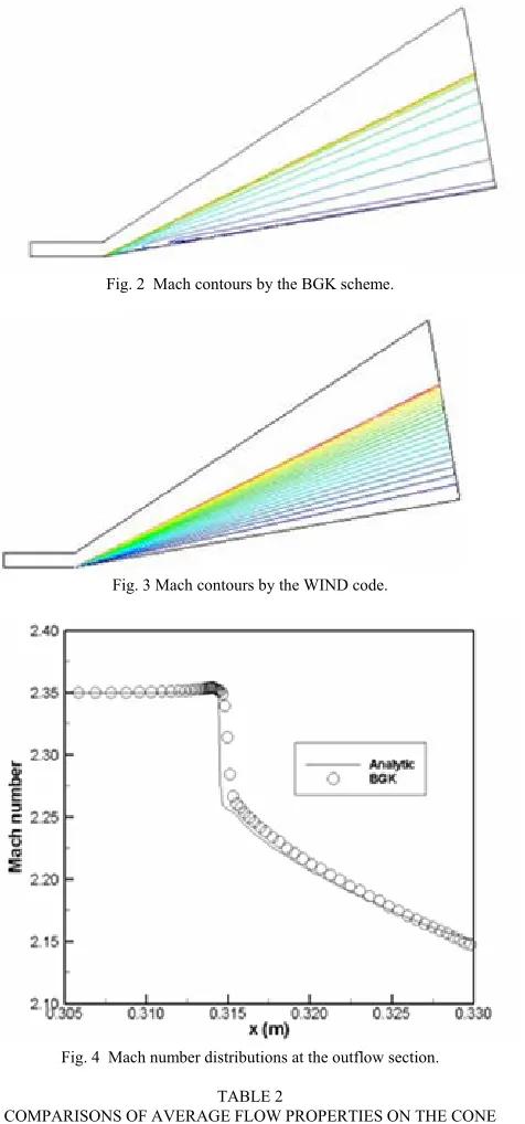
e.g. [17]. A sample of these analytical solutions obtained via the mentioned differential equations is contained in Table 1. The subscript 1 refers to the free stream conditions. The subscript 2 refers to the conditions behind the shock. The subscript 3 refers to the conditions on the surface of the cone. The angle of the shock is 27.18 degrees. In addition, comparisons are also made between the results of the BGK flow solver with WIND code from NPARC (National Project for Application-oriented Research in CFD) Alliance to assess the computational characteristics of the developed flow solver. The Mach number contour plots of the flow over the cone predicted by the BGK flow solver is shown in Fig. 2. Comparing this result with the prediction by the WIND code as shown in Fig. 3, it can be observed that both results are comparable to each others. Figure 4 shows the Mach number distributions taken at the outflow section of the flow field domain, i.e. at the right-side plane. In this figure, the computed Mach number by the BGK flow solver is compared against the analytic data and illustrated that a very good agreement is achieved. However, the predicted shock location is about a step downstream of the domain compared to the actual location. Also from the figure, the value of the Mach number (i.e. M2) predicted by the BGK flow solver after the shock is about 2.2667. Comparing this value against the analytical value, it has about 0.03 % error which can be considered relatively very low. In Table 2, the average flow properties calculated along the surface of the cone which simply sums up the values after x of 0.06 m and averages them, where the values obtained, should be fairly constant. In addition, the percentage of errors generated by the two numerical flow solvers against the analytical data is also shown in the same table. By comparing the various results contained in the table, the errors produced by both solvers are marginally the same, with WIND showing better accuracy for the Mach number and pressure properties, while the BGK proved to have a better resolution in terms of temperature property. Even so, the value of the errors produced by both solvers is significantly very low. Hence, this would imply that the BGK solver is able to provide good resolution of the flow along the surface of the cone.
B. Normal Shock at Mach 1.3
This flow problem would serve as the subsequent verification case involving steady, inviscid, adiabatic flow at Mach 1.3 with formation of a normal shock in the flow field where supersonic flow enters the normal shock and subsonic flow exits the shock. This flow is a classic, fundamental supersonic flow whose analytic solution is exact and can be found in any compressible flow textbook, such as the book by Anderson [17].
The flow conditions at the free stream described for the initiation of the computation are set as follows: Mach number M∞ = 1.3, pressure p∞ = 68947.57 Pa, temperature T∞ = 288.89 K and reference length L∞ = 0.3048 m. The
computational domain for this flow problem has a size of 202 by 11 by 5 grid points and the generated mesh is shown in Fig. 5. As for the enforcement of boundary conditions, the following conditions are stated: the left- and top-side planes are free stream; the bottom-, front-, and rear-side planes are inviscid wall; and the right-side plane is subsonic
outflow with prescribed Mach number (i.e. M = 0.876). The predicted Mach contours by the BGK flow solver is shown in Fig. 6, which is identical to the one produced by [18]. The resolution of the Mach number by the solver at the bottom wall of the flow field domain is determined and contained in Fig. 7. Through this figure, the predicted shock location is clearly shown to be placed at the desired location, i.e. x = 0.3048 m. It also revealed that the distribution of the Mach number produced by the BGK flow solver is of high quality where the resolution of the flow property, especially near the vicinity of the shock is captured without any numerical instability such as pre- or post-shock oscillation. Table 3 presents the analytic solutions for a Mach 1.3 supersonic flow through a normal shock [18], where the subscript 1 refers to the supersonic side of the shock and subscript 2 refers to the subsonic side of the shock. While in Table 4, it contains the average flow properties calculated along the bottom surface of the flow domain which simply sums up the values after x of 0.36576 m and averages them, which should be fairly constant. The purpose of Table 4 is to compare the numerical results and their respective percentage of errors from the analytical values (i.e. Table 3) for the two flow solvers i.e. BGK and WIND, respectively. From the comparisons, the errors produced by both solvers are marginally the same with the BGK shown to have a better accuracy in predicting the flow field. Even so, the values of the errors produced by both solvers are significantly low.
V. CONCLUSION
In this paper, a numerical flow solver based on the BGK scheme has been successfully developed to compute three-dimensional compressible inviscid flow. Two benchmark cases of this flow realm have been chosen to assess and to validate the computational results of the developed flow solver. The findings for the test cases as recorded in this paper clearly show that the BGK flow solver is able to provide a very good resolution of the flow which contains complex shock waves formation with reflections. This claim is substantiated by comparing the numerical results against available analytical solutions and published numerical results (i.e. WIND). In brief, this paper concludes that the BGK scheme formulated via the finite difference method is an accurate and robust numerical scheme for computing three-dimensional compressible inviscid flow.
VI. ACKNOWLEDGMENTS
The authors would like to acknowledge the support of the International Islamic University Malaysia (IIUM) through Research Management Center under the grant No. EDW B-0805-140.
REFERENCES
[1] Pullin, D. I., “Direct Simulation Methods for Compressible Inviscid Ideal Gas Flow,” J. Comp. Phys., Vol. 34, 1980, pp. 231-244. [2] Mandal, J. C. and Deshpande, S. M., “Kinetic Flux Vector Splitting
for Euler Equations,” Comp. Fluids, Vol. 23, No. 2, 1994, pp. 447-478.
[4] Xu, K., “Gas-Kinetic Theory Based Flux Splitting Method for Ideal Magnetohydrodynamics,” J. Comp. Phys., Vol. 153, No. 2, 1999, pp. 334-352.
[5] Chae, D. S., Kim, C. A. and Rho, O. H., “Development of an Improved Gas-Kinetic BGK Scheme for Inviscid and Viscous Flows,”
J. Comp. Phys., Vol. 158, 2000, pp. 1-27.
[6] Ong, J. C., Omar, A. A., Asrar, W. and Hamdan, M. M., “An Implicit Gas-Kinetic BGK Scheme for Two-Dimensional Compressible Inviscid Flows,” AIAA Journal, Vol. 42, No. 7, 2004, pp 1293-1301. [7] Ong, J. C., Omar, A. A., Asrar W. and Zaludin, Z. A., “Hypersonic
Flow Simulation By The Gas-Kinetic BGK Scheme,” AIAA Journal, Vol. 43, No. 7, 2005, pp 1427-1433.
[8] Zhang, S. Q., Ghidaoui, M. S., Gray, W. G. and Li, N. Z., “A Kinetic Flux Vector Splitting Scheme for Shallow Water Flows,” Advances in Water Resources, Vol. 26, 2003, pp. 635-647.
[9] Xu, K., Mao, M. and Tang, L., “A Multidimensional Gas-Kinetic BGK Scheme for Hypersonic Viscous Flow,” J. Comp. Phys., Vol. 203, No. 2, 2005, pp. 405-421.
[10] May, G., Srinivasan, B. and Jameson, A., “An Improved Gas-Kinetic BGK Finite-Volume Method for Three-Dimensional Transonic Flow,” J. Comp. Phys., Vol. 220, No. 2, 2007, pp. 856-878.
[11] Ilgaz, M. and Tuncer, I. H., “A Gas-Kinetic BGK Scheme for Parallel Solution of 3-D Viscous Flows on Unstructured Hybrid Grids,” 18th AIAA Computational Fluid Dynamics Conference, AIAA Paper 2007-4582, Miami, Florida, 2007.
[12] Ravichandran, K. S., “Higher Order KFVS Algorithms using Compact Upwind Difference Operators,” J. Comp. Phys., Vol. 130, No. 2, 1997, pp. 322-334.
[13] Omar, A. A., Ong J. C., Lim J. H. and Asrar W., “Finite Difference Gas-Kinetic BGK Scheme for Compressible Inviscid Flow Computation”, Int. J. of Comp. Fluid Dynamics, Vol. 22, No. 3, 2008, pp. 183-192.
[14] Omar A. A., Ong J. C., Asrar W. and Ismail A. F., “Accuray of Bhatnagaar-Gross-Krook Scheme in Solving Laminar Viscous Flow Problems,” AIAA Journal, Vol. 47, No. 4, 2009, pp. 885-892. [15] Hoffmann, K. A. and Chiang, S. T., “Computational Fluid Dynamics
for Engineers,” Engineering Education System, Wichita, Vol. 2, chap. 11 and 14, 1993.
[16] Hirsch C., “The Numerical Computation of Internal and External Flows,” John Wiley & Sons, New York, Vol. 2, Chap. 21, 1990. [17] Anderson, J. D., “Modern Compressible Flow,” McGraw Hill Inc.,
New York, 1982.
[18] Slater, J. W., “Normal Shock at Mach 1.3,” NPARC Alliance Validation Archive [online database], URL:
http://www.grc.nasa.gov/WWW/wind/valid/normal/normal.html [cited 9 July 2009].
Fig. 1 Computational mesh generated for the 10 degrees cone at Mach 2.35.
TABLE 1
ANALYTICAL SOLUTION FOR THE 10 DEGREES CONE AT MACH 2.35
Property 2 3
M 2.2677 2.1469
p / p1 1.1781 1.4234
T / T1 1.0481 1.1063
[image:5.612.66.550.13.742.2]ρ / ρ1 1.1240 1.2867
Fig. 2 Mach contours by the BGK scheme.
Fig. 3 Mach contours by the WIND code.
Fig. 4 Mach number distributions at the outflow section.
TABLE 2
COMPARISONS OF AVERAGE FLOW PROPERTIES ON THE CONE SURFACE
Solver M3 Error
%
p3 / p1 Error %
T3 / T1 Error % BGK 2.14788
3
0.0458 1.36996 3.7545 1.10945 3
0.2850
WIND 2.14674 9
0.0070 1.37410 0
3.4635 1.09514 1
1.0087
[image:5.612.314.552.47.556.2]Fig. 6 Mach contours by BGK scheme.
[image:6.612.72.316.56.408.2]Fig. 7 Mach number distribution along the bottom wall.
TABLE 3
ANALYTICAL SOLUTION FOR THE NORMAL SHOCK AT MACH 1.3
Property Exact
M2 0.7860
p2 / p1 1.8050
T2 / T1 1.1909
ρ2 / ρ1 1.5157
TABLE 4
COMPARISONS OF AVERAGE FLOW PROPERTIES ON THE BOTTOM SURFACE OF NORMAL SHOCK TEST CASE
Solver M2 Error
%
p2 / p1 Error % T2 / T1 Error % BGK 0.78600
9
0.001 1
1.80500 1
0.00006 2
1.19086 9
0.002 6 WIND 0.78598
9
0.001 4
1.80490 6
0.0052 1.19085 7