CODRA: A Novel Discriminative Framework for Rhetorical Analysis

for Rhetorical Analysis

Shafiq Joty

Qatar Computing Research Institute

Giuseppe Carenini

Raymond T. Ng

University of British Columbia

Clauses and sentences rarely stand on their own in an actual discourse; rather, the relationship between them carries important information that allows the discourse to express a meaning as a whole beyond the sum of its individual parts. Rhetorical analysis seeks to uncover this coherence structure. In this article, we present CODRA— a COmplete probabilistic Discriminative framework for performing Rhetorical Analysis in accordance with Rhetorical Structure Theory, which posits a tree representation of a discourse.

CODRA comprises a discourse segmenter and a discourse parser. First, the discourse segmenter, which is based on a binary classifier, identifies the elementary discourse units in a given text. Then the discourse parser builds a discourse tree by applying an optimal parsing algorithm to probabilities inferred from two Conditional Random Fields: one for intra-sentential parsing and the other for multi-sentential parsing. We present two approaches to combine these two stages of parsing effectively. By conducting a series of empirical evaluations over two different data sets, we demonstrate thatCODRAsignificantly outperforms the state-of-the-art, often by a wide margin. We also show that a reranking of the k-best parse hypotheses generated byCODRAcan potentially improve the accuracy even further.

1. Introduction

A well-written text is not merely a sequence of independent and isolated sentences, but instead a sequence of structured and related sentences, where the meaning of a sentence relates to the previous and the following ones. In other words, a well-written

∗Arabic Language Technologies, Qatar Computing Research Institute, Qatar Foundation, Doha, Qatar. E-mail:[email protected].

∗∗Computer Science Department, University of British Columbia, Vancouver, BC, Canada, V6T 1Z4. E-mail:[email protected].

†Computer Science Department, University of British Columbia, Vancouver, BC, Canada, V6T 1Z4. E-mail:[email protected].

Submission received: 11 May 2014; revised version received: 29 January 2015; accepted for publication: 18 March 2015.

text has acoherence structure(Halliday and Hasan 1976; Hobbs 1979), which logically binds its clauses and sentences together to express a meaning as a whole. Rhetorical analysisseeks to uncover this coherence structure underneath the text; this has been shown to be beneficial for many Natural Language Processing (NLP) applications, including text summarization and compression (Marcu 2000b; Daum´e and Marcu 2002; Sporleder and Lapata 2005; Louis, Joshi, and Nenkova 2010), text generation (Prasad et al. 2005), machine translation evaluation (Guzm´an et al. 2014a, 2014b; Joty et al. 2014), sentiment analysis (Somasundaran 2010; Lazaridou, Titov, and Sporleder 2013), information extraction (Teufel and Moens 2002; Maslennikov and Chua 2007), and question answering (Verberne et al. 2007). Furthermore, rhetorical structures can be useful for other discourse analysis tasks, including co-reference resolution using Veins theory (Cristea, Ide, and Romary 1998).

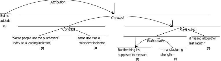
Different formal theories of discourse have been proposed from different view-points to describe the coherence structure of a text. For example, Martin (1992) and Knott and Dale (1994) propose discourse relations based on the usage of discourse connectives (e.g., because, but) in the text. Asher and Lascarides (2003) propose Seg-mented Discourse Representation Theory, which is driven by sentence semantics. Webber (2004) and Danlos (2009) extend sentence grammar to formalize discourse struc-ture.Rhetorical Structure Theory (RST), proposed by Mann and Thompson (1988), is perhaps the most influential theory of discourse in computational linguistics. Although it was initially intended to be used in text generation, later it became popular as a frame-work for parsing the structure of a text (Taboada and Mann 2006). RST represents texts by labeled hierarchical structures, called Discourse Trees (DTs). For example, consider the DT shown in Figure 1 for the following text:

But he added: “Some people use the purchasers’ index as a leading indicator, some use it as a coincident indicator. But the thing it’s supposed to measure—manufacturing strength—it missed altogether last month.”

The leaves of a DT correspond to contiguous atomic text spans, calledelementary discourse units (EDUs; six in the example). EDUs are clause-like units that serve as building blocks. Adjacent EDUs are connected by coherence relations (e.g.,Elaboration,

Contrast), forming larger discourse units (represented by internal nodes), which in turn are also subject to this relation linking. Discourse units linked by a rhetorical relation are

But he added:

"Some people use the purchasers’ index as a leading indicator,

some use it as a coincident indicator.

But the thing it’s supposed to measure

-- manufacturing strength

--it missed altogether last month." <P> Elaboration

Same-Unit Contrast

Contrast Attribution

(1)

(2) (3)

(4) (5)

(6)

Figure 1

further distinguished based on their relative importance in the text:nucleiare the core parts of the relation andsatellitesare peripheral or supportive ones. For example, in Figure 1,Elaborationis a relation between a nucleus (EDU 4) and a satellite (EDU 5), and Contrast is a relation between two nuclei (EDUs 2 and 3). Carlson, Marcu, and Okurowski (2002) constructed the first large RST-annotated corpus (RST–DT) onWall Street Journalarticles from the Penn Treebank. Whereas Mann and Thompson (1988) had suggested about 25 relations, the RST–DT uses 53 mono-nuclear and 25 multi-nuclear relations. The relations are grouped into 16 coarse-grained categories; see Carlson and Marcu (2001) for a detailed description of the relations. Conventionally, rhetorical anal-ysis in RST involves two subtasks:discourse segmentationis the task of breaking the text into a sequence of EDUs, anddiscourse parsingis the task of linking the discourse units (EDUs and larger units) into a labeled tree. In this article, we use the termsdiscourse parsingandrhetorical parsinginterchangeably.

While recent advances in automatic discourse segmentation have attained high accuracies (an F-score of 90.5% reported by Fisher and Roark [2007]), discourse parsing still poses significant challenges (Feng and Hirst 2012) and the performance of the exist-ing discourse parsers (Soricut and Marcu 2003; Subba and Di-Eugenio 2009; Hernault et al. 2010) is still considerably inferior compared with the human gold standard. Thus, the impact of rhetorical structure in downstream NLP applications is still very limited. The work we present in this article aims to reduce this performance gap and take discourse parsing one step further. To this end, we address three key limitations of existing discourse parsers.

First, existing discourse parsers typically model the structure and the labels of a DT separately, and also do not take into account the sequential dependencies between the DT constituents. However, for several NLP tasks, it has recently been shown that joint models typically outperform independent or pipeline models (Murphy 2012, page 687). This is also supported in a recent study by Feng and Hirst (2012), in which the performance of a greedy bottom–up discourse parser improved when sequential de-pendencies were considered by usinggoldannotations for the neighboring (i.e., previous and next) discourse units as contextual features in the parsing model. To address this limitation of existing parsers, as the first contribution, we propose a novel discourse parser based on probabilistic discriminative parsing models, expressed as Conditional Random Fields (CRFs) (Sutton, McCallum, and Rohanimanesh 2007), to infer the proba-bility of all possible DT constituents. The CRF models effectively represent the structure and the label of a DT constituent jointly, and, whenever possible, capture the sequential dependencies.

Second, existing discourse parsers typically apply greedy and sub-optimal parsing algorithms to build a DT. To cope with this limitation, we use the inferred (posterior) probabilities from our CRF parsing models in a probabilistic CKY-like bottom–up parsing algorithm (Jurafsky and Martin 2008), which is non-greedy and optimal. Furthermore, a simple modification of this parsing algorithm allows us to generate

k-best (i.e., the khighest probability) parse hypotheses for each input text that could then be used in arerankerto improve over the initial ranking using additional (global) features of the discourse tree as evidence, a strategy that has been successfully explored in syntactic parsing (Charniak and Johnson 2005; Collins and Koo 2005).

are distributed differently intra-sententially versus multi-sententially. Also, they could independently choose their own informative feature sets. As another key contribution of our work, we devise two different parsing components: one for intra-sentential parsing, the other for multi-sentential parsing. This provides for scalable, modular, and flexible solutions that can exploit the strong correlation observed between the text structure (i.e., sentence boundaries) and the structure of the discourse tree.

In order to develop a complete and robust discourse parser, we combine our intra-sentential and multi-intra-sentential parsing components in two different ways. Because most sentences have a well-formed discourse sub-tree in the full DT (e.g., the second sentence in Figure 1), our first approach constructs a DT for every sentence using our intra-sentential parser, and then runs the multi-intra-sentential parser on the resulting sentence-level DTs to build a complete DT for the whole document. However, this approach would fail in those cases where discourse structures violate sentence boundaries, also called “leaky” boundaries (Vliet and Redeker 2011). For example, consider the first sentence in Figure 1. It does not have a well-formed discourse sub-tree because the unit containing EDUs 2 and 3 merges with the next sentence and only then is the resulting unit merged with EDU 1. Our second approach, in order to deal with these leaky cases, builds sentence-level sub-trees by applying the intra-sentential parser on a sliding window covering two adjacent sentences and by then consolidating the results produced by overlapping windows. After that, the multi-sentential parser takes all these sentence-level sub-trees and builds a full DT for the whole document.

Our discourse parser assumes that the input text has already been segmented into elementary discourse units. As an additional contribution, we propose a novel discriminative approach to discourse segmentation that not only achieves state-of-the-art performance, but also reduces time and space complexities by using fewer features. Notice that the combination of our segmenter with our parser forms a COmplete probabilistic Discriminative framework for Rhetorical Analysis (CODRA).

Whereas previous systems have been tested on only one corpus, we evaluate our framework on texts from two very different genres: news articles and instructional how-to manuals. The results demonstrate that our approach how-to discourse parsing provides consistent and statistically significant improvements over previous methods both at the sentence level and at the document level. The performance of our final system compares very favorably to the performance of state-of-the-art discourse parsers. Finally, the oracle accuracy computed based on thek-best parse hypotheses generated by our parser demonstrates that a reranker could potentially improve the accuracy further.

After discussing related work in Section 2, we present our rhetorical analysis frame-work in Section 3. In Section 4, we describe our discourse parser. Then, in Section 5 we present our discourse segmenter. The experiments and analysis of results are presented in Section 6. Finally, we summarize our contributions with future directions in Section 7.

2. Related Work

2.1 Unsupervised and Rule-Based Approaches

Although the most effective approaches to rhetorical analysis to date rely on supervised machine learning methods trained on human-annotated data, unsupervised methods have also been proposed, as they do not require human-annotated data and can be more easily applied to new domains.

Often, discourse connectives likebut, because,andalthoughconvey clear information on the kind of relation linking the two text segments. In his early work, Marcu (2000a) presented a shallow rule-based approach relying on discourse connectives (or cues) and surface patterns. He used hand-coded rules, derived from an extensive corpus study, to break the text into EDUs and to build DTs for sentences first, then for paragraphs, and so on. Despite the fact that this work pioneered the field of rhetorical analysis, it has many limitations. First, identifying discourse connectives is a difficult task on its own, because (depending on the usage), the same phrase may or may not signal a discourse relation (Pitler and Nenkova 2009). For example, but can either signal a

Contrastdiscourse relation or can simply perform non-discourse acts. Second, discourse segmentation using only discourse connectives fails to attain high accuracy (Soricut and Marcu 2003). Third, DT structures do not always correspond to paragraph structures; for example, Sporleder and Lapata (2004) report that more than 20% of the paragraphs in the RST–DT corpus (Carlson, Marcu, and Okurowski 2002) do not correspond to a discourse unit in the DT. Fourth, discourse cues are sometimes ambiguous; for example,

butcan signalContrast, AntithesisandConcession, and so on.

Finally, a more serious problem with the rule-based approach is that often rhetorical relations are not explicitly signaled by discourse cues. For example, in RST–DT, Marcu and Echihabi (2002) found that only 61 out of 238 Contrast relations and 79 out of 307Cause–Explanationrelations were explicitly signaled by cue phrases. In the British National Corpus, Sporleder and Lascarides (2008) report that half of the sentences lack a discourse cue. Other studies (Schauer and Hahn 2001; Stede 2004; Taboada 2006; Subba and Di-Eugenio 2009) report even higher figures: About 60% of discourse relations are not explicitly signaled. Therefore, rather than relying on hand-coded rules based on discourse cues and surface patterns, recent approaches usemachine learningtechniques with a large set of informative features.

While some rhetorical relations need to be explicitly signaled by discourse cues (e.g.,Concession) and some do not (e.g., Background), there is a large middle ground of relations that may be signaled or not. For these “middle ground” relations, can we exploit features present in the signaled cases to automatically identify relations when they are not explicitly signaled? The idea is to use unambiguous discourse cues (e.g.,

althoughfor Contrast,for examplefor Elaboration) to automatically label a large corpus with rhetorical relations that could then be used to train a supervised model.1

A series of previous studies have explored this idea. Marcu and Echihabi (2002) first attempted to identify four broad classes of relations:Contrast, Elaboration, Condition,

andCause–Explanation–Evidence. They used a naive Bayes classifier based on word pairs (w1,w2), where w1 occurs in the left segment, and w2 occurs in the right segment. Sporleder and Lascarides (2005) included other features (e.g., words and their stems, Part-of-Speech [POS] tags, positions, segment lengths) in a boosting-based classifier (i.e., BoosTexter [Schapire and Singer 2000]) to further improve relation classification accuracy. However, these studies evaluated classification performance on the instances

where rhetorical relations were originally signaled (i.e., the discourse cues were artifi-cially removed), and did not verify how well this approach performs on the instances that are not originally signaled. Subsequent studies (Blair-Goldensohn, McKeown, and Rambow 2007; Sporleder 2007; Sporleder and Lascarides 2008) confirm that classifiers trained on instances stripped of their original discourse cues do not generalize well to implicit cases because they are linguistically quite different.

Note that this approach to identifying discourse relations in the absence of manually labeled data does not fully solve the parsing problem (i.e., building DTs); rather, it only attempts to identify a small subset of coarser relations between two (flat) text segments (i.e., a tagging problem). Arguably, to perform a complete rhetorical analysis, one needs to use supervised machine learning techniques based on human-annotated data.

2.2 Supervised Approaches

Marcu (1999) applies supervised machine learning techniques to build a discourse segmenter and a shift–reduce discourse parser. Both the segmenter and the parser rely on C4.5 decision tree classifiers (Poole and Mackworth 2010) to learn the rules auto-matically from the data. The discourse segmenter mainly uses discourse cues, shallow-syntactic (i.e., POS tags) and contextual features (i.e., neighboring words and their POS tags). To learn the shift–reduce actions, the discourse parser encodes five types of features: lexical (e.g., discourse cues), shallow-syntactic, textual similarity, operational (previousnshift–reduce operations), and rhetorical sub-structural features. Despite the fact that this work has pioneered many of today’s machine learning approaches to discourse parsing, it has all the limitations mentioned in Section 1.

The work of Marcu (1999) is considerably improved by Soricut and Marcu (2003). They present the publicly available SPADE system,2 _{which comes with probabilistic} models for discourse segmentation andsentence-leveldiscourse parsing. Their segmen-tation and parsing models are based on lexico-syntactic patterns (or features) extracted from the lexicalized syntactic tree of a sentence. The discourse parser uses an optimal parsing algorithm to find the most probable DT structure for a sentence. SPADE was trained and tested on the RST–DT corpus. This work, by showing empirically the connection between syntax and discourse structure at the sentence level, has greatly in-fluenced all major contributions in this area ever since. However, it is limited in several ways. First, SPADE does not produce a full-text (i.e., document-level) parse. Second, it applies agenerativeparsing model based on only lexico-syntactic features, whereas dis-criminative models are generally considered to be more accurate, and can incorporate arbitrary features more effectively (Murphy 2012). Third, the parsing model makes an independence assumption between the label and the structure of a DT constituent, and it ignores the sequential and the hierarchical dependencies between the DT constituents. Subsequent research addresses the question of how much syntax one really needs in rhetorical analysis. Sporleder and Lapata (2005) focus on thediscourse chunking prob-lem, comprising two subtasks: discourse segmentation and (flat) nuclearity assignment. They formulate discourse chunking in two alternative ways. First,one-step classifica-tion, where the discourse chunker, a multi-class classifier, assigns to each token one of the four labels: (1) B–NUC (beginning of a nucleus), (2) I–NUC (inside a nucleus), (3) B– SAT (beginning of a satellite), and (4) I–SAT (inside a satellite). Therefore, this approach performs discourse segmentation and nuclearity assignment simultaneously. Second,

two-step classification, where in the first step, the discourse segmenter (a binary clas-sifier) labels each token as either B (beginning of an EDU) or I (inside an EDU). Then, in the second step, a nuclearity labeler (another binary classifier) assigns a nuclearity status to each segment. The two-step approach avoids illegal chunk sequences like a B–NUC followed by an I–SAT or a B–SAT followed by an I–NUC, and in this approach, it is easier to incorporate sentence-level properties like the constraint that a sentence must contain at least one nucleus. They examine whether shallow-syntactic features (e.g., POS and phrase tags) would be sufficient for these purposes. The evaluation on the RST–DT shows that the two-step approach outperforms the one-step approach, and its performance is comparable to that of SPADE, which requires relatively expensive full syntactic parses.

In follow–up work, Fisher and Roark (2007) demonstrate over 4% absolute perfor-mance gain in discourse segmentation, by combining the features extracted from the syntactic tree with the ones derived via POS tagging and shallow syntactic parsing (i.e., chunking). Using quite a large number of features in a binary log-linear model, they achieve state-of-the-art performance in discourse segmentation on the RST–DT test set.

In a different approach, Regneri, Egg, and Koller (2008) propose to use Underspec-ified Discourse Representation (UDR)as an intermediate representation for discourse parsing. Underspecified representations offer a single compact representation to express possible ambiguities in a linguistic structure, and have been primarily used to deal with scope ambiguity in semantic structures (Reyle 1993; Egg, Koller, and Niehren 2001; Althaus et al. 2003; Koller, Regneri, and Thater 2008). Assuming that a UDR of a DT is already given in the form of a dominance graph (Althaus et al. 2003), Regneri, Egg, and Koller (2008) convert it into a more expressive and complete UDR representation called regular tree grammar (Koller, Regneri, and Thater 2008), for which efficient algorithms (Knight and Graehl 2005) already exist to derive the best configuration (i.e., the best discourse tree).

Hernault et al. (2010) present the publicly availableHILDAsystem,3_{which comes} with a discourse segmenter and a parser based on Support Vector Machines (SVMs). The discourse segmenter is a binary SVM classifier that uses the same lexico-syntactic features used in SPADE, but with more context (i.e., the lexico-syntactic features for the previous two words and the following two words). The discourse parser itera-tively uses two SVM classifiers in a pipeline to build a DT. In each iteration, a binary classifier first decides which of the adjacent units to merge, then a multi-class classi-fier connects the selected units with an appropriate relation label. Using this simple method, they report promising results in document-level discourse parsing on the RST–DT.

For a different genre, instructional texts, Subba and Di-Eugenio (2009) propose a shift–reduce discourse parser that relies on a classifier for relation labeling. Their clas-sifier usesInductive Logic Programming (ILP)to learn first-order logic rules from a large set of features including the linguistically richcompositional semanticscoming from a semantic parser. They demonstrate that including compositional semantics with other features improves the performance of the classifier, thus, also improves the performance of the parser.

Both HILDA and the ILP-based approach of Subba and Di-Eugenio (2009) are lim-ited in several ways. First, they do not differentiate between intra- and multi-sentential

parsing, and both scenarios use a single uniform parsing model. Second, they take a greedy (i.e., sub-optimal) approach to construct a DT. Third, they disregard sequential dependencies between DT constituents. Furthermore, HILDA considers the structure and the labels of a DT separately. Our discourse parser CODRA, as described in the next section, addresses all these limitations.

More recent work than ours also attempts to address some of the above-mentioned limitations of the existing discourse parsers. Similar to us, Feng and Hirst (2014) gen-erate a document-level DT in two stages, where a multi-sentential parsing follows an intra-sentential one. At each stage, they iteratively use two separate linear-chain CRFs (Lafferty, McCallum, and Pereira 2001) in a cascade: one for predicting the presence of rhetorical relations between adjacent discourse units in a sequence, and the other to predict the relation label between the two most probable adjacent units to be merged as selected by the previous CRF. While they use CRFs to take into account the sequen-tial dependencies between DT constituents, they use them greedily during parsing to achieve efficiency. They also propose a greedypost-editingstep based on an additional feature (i.e., depth of a discourse unit) to modify the initial DT, which gives them a significant gain in performance. In a different approach, Li et al. (2014) propose a discourse-level dependency structure to capture direct relationships between EDUs rather than deep hierarchical relationships. They first create a discourse dependency treebank by converting thedeepannotations in RST–DT to shallowhead-dependent anno-tations between EDUs. To find the dependency parse (i.e., an optimal spanning tree) for a given text, they apply Eisner (1996) and Maximum Spanning Tree (McDonald et al. 2005) dependency parsing algorithms with the Margin Infused Relaxed Algorithm online learning framework (McDonald, Crammer, and Pereira 2005).

With the successful application of deep learningto numerous NLP problems in-cluding syntactic parsing (Socher et al. 2013a), sentiment analysis (Socher et al. 2013b), and various tagging tasks (Collobert et al. 2011), a couple of recent studies in discourse parsing also use deep neural networks (DNNs) and related feature representation meth-ods. Inspired by the work of Socher et al. (2013a, 2013b), Li, Li, and Hovy (2014) propose a recursive DNN for discourse parsing. However, as in Socher et al. (2013a, 2013b), word vectors (i.e., embeddings) are not learned explicitly for the task, rather they are taken from Collobert et al. (2011). Given the vectors of the words in an EDU, their model first composes them hierarchically based on a syntactic parse tree to get the vector representation for the EDU. Adjacent discourse units are then merged hierarchically to get the vector representations for the higher order discourse units. In every step, the merging is done using one binary (structure) and one multi-class (relation) classifier, each having a three-layer neural network architecture. The cost function for training the model is given by these two cascaded classifiers applied at different levels of the DT. Similar to our method, they use the classifier probabilities in a CKY-like parsing algorithm to find the global optimal DT. Finally, Ji and Eisenstein (2014) present a feature representation learning method in a shift–reduce discourse parser (Marcu 1999). Unlike DNNs, which learn non-linear feature transformations in a maximum likelihood model, they learn linear transformations of features in a max margin classification model.

3. Overview of Our Rhetorical Analysis Framework

model Algorithm Sentences

segmented into EDUs

Document-level discourse tree

Intra-sentential parser

Multi-sentential parser

model Algorithm

Segmentation model

Segmenter Parser

Document

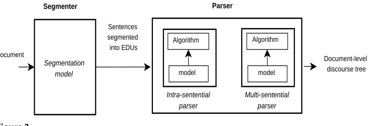
Figure 2

CODRA architecture.

is shown in Appendix A.4 _{The color of a node represents its nuclearity status: blue} denoting nucleus and yellow denoting satellite. The demo also allows some useful user interactions—for example, collapsing or expanding a node, highlighting an EDU, and so on.5

CODRA follows a pipeline architecture, shown in Figure 2. Given a raw text, the first task in the rhetorical analysis pipeline is to break the text into a sequence of EDUs (i.e., discourse segmentation). Because it is taken for granted that sentence bound-aries are also EDU boundbound-aries (i.e., EDUs do not span across multiple sentences), the discourse segmentation task boils down to finding EDU boundaries inside sentences. CODRA uses amaximum entropymodel for discourse segmentation (see Section 5).

Once the EDUs are identified, the discourse parsing problem is determining which discourse units (EDUs or larger units) to relate (i.e., the structure), and what relations (i.e., the labels) to use in the process of building the DT. Specifically, discourse parsing requires: (1)a parsing model to explore the search space of possible structures and labels for their nodes, and (2)a parsing algorithmfor selecting the best parse tree(s) among the candidates. A probabilistic parsing model like ours assigns a probability to every possible DT. The parsing algorithm then picks the most probable DTs.

The existing discourse parsers (Marcu 1999; Soricut and Marcu 2003; Subba and Di-Eugenio 2009; Hernault et al. 2010) described in Section 2 use parsing models that disregard the structural interdependencies between the DT constituents. However, we hypothesize that, like syntactic parsing, discourse parsing is also a structured predic-tion problem, which involves predicting multiple variables (i.e., the structure and the relation labels) that depend on each other (Smith 2011). Recently, Feng and Hirst (2012) also found these interdependencies to be critical for parsing performance. To capture the structural dependencies between the DT constituents, CODRA uses undirected conditional graphical models (i.e., CRFs) as its parsing models.

To find the most probable DT, unlike most previous studies (Marcu 1999; Subba and Di-Eugenio 2009; Hernault et al. 2010), which adopt a greedy solution, CODRA applies an optimal CKY parsing algorithm to the inferred posterior probabilities (obtained from the CRFs) of all possible DT constituents. Furthermore, the parsing algorithm allows CODRA to generate a list ofk-best parse hypotheses for a given text.

4 The demo of CODRA is available athttp://109.228.0.153/Discourse Parser Demo/.

The source code of CODRA is available fromhttp://alt.qcri.org/tools/.

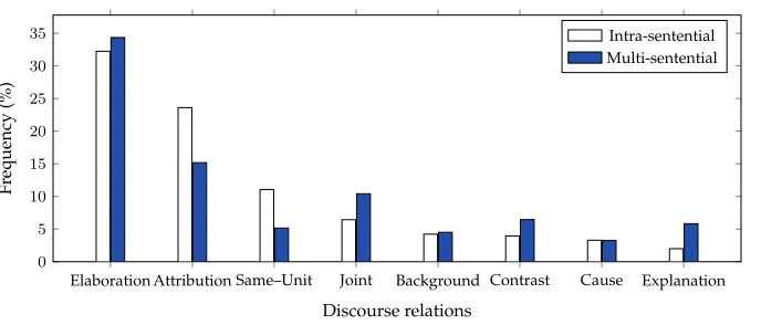
Figure 3

Distributions of the eight most frequent relations in intra-sentential and multi-sentential parsing scenarios on the RST–DT training set.

Note that the way CRFs and CKY are used in CODRA is quite different from the way they are used in syntactic parsing. For example, in the CRF-based constituency parsing proposed by Finkel, Kleeman, and Manning (2008), the conditional probability distribution of a parse tree given a sentence decomposes across factors defined over

productions, and the standardinside–outsidealgorithm is used for inference on possible trees. In contrast, CODRA first uses the standard forward–backward algorithm in a “fat” chain structured6_{CRF (to be discussed in Section 4.1.1) to compute the posterior} probabilities of all possible DT constituents for a given text (i.e., EDUs); then it uses a CKY parsing algorithm to combine those probabilities and find the most probable DT.

Another crucial question related to parsing models is whether to use a single model or two different models for parsing at the sentence-level (i.e., intra-sentential) and at the document-level (i.e., multi-sentential). A simple and straightforward strategy would be to use a single unified parsing model for both intra- and multi-sentential parsing without distinguishing the two cases, as was previously done (Marcu 1999; Subba and Di-Eugenio 2009; Hernault et al. 2010). That approach has the advantages of making the parsing process easier, and the model gets more data to learn from. However, for a solution like ours, which tries to capture the interdependencies between constituents, this would be problematic with respect to scalability and inappropriate because of two modeling issues.

More specifically, for scalability note that the number of valid trees grows exponen-tially with the number of EDUs in a document.7 _{Therefore, an exhaustive search over} all the valid DTs is often infeasible, even for relatively small documents.

For modeling, a single unified approach is inappropriate for two reasons. On the one hand, it appears that discourse relations are distributed differently intra- versus multi-sententially. For example, Figure 3 shows a comparison between the two dis-tributions of the eight most frequent relations in the RST–DT training set. Notice that

Same–Unitis more frequent thanJointin the intra-sentential case, whereasJointis more frequent thanSame–Unitin the multi-sentential case. Similarly, the relative distributions

6 By the term “fat” we refer to CRFs with multiple (interconnected) chains of output variables.

ofBackground,Contrast,Cause, andExplanationare different in the two parsing scenarios. On the other hand, different kinds of features are applicable and informative for intra-versus multi-sentential parsing. For example, syntactic features likedominance sets (Soricut and Marcu 2003) are extremely useful for parsing at the sentence-level, but are not even applicable in the multi-sentential case. Likewise, lexical chain features (Sporleder and Lapata 2004), which are useful for multi-sentential parsing, are not applicable at the sentence level.

Based on these above observations, CODRA comprises two separate modules: an intra-sentential parserand amulti-sentential parser, as shown in Figure 2. First, the intra-sentential parser produces one or more discourse sub-trees for each sentence. Then, the multi-sentential parser generates a full DT for the document from these sub-trees. Both of our parsers have the same two components: aparsing modeland a

parsing algorithm. Whereas the two parsing models are rather different, the same parsing algorithm is shared by the two modules. Staging multi-sentential parsing on top of intra-sentential parsing in this way allows CODRA to explicitly exploit the strong correlation observed between the text structure and the DT structure, as explained in detail in Section 4.3.

4. The Discourse Parser

Before describing the parsing models and the parsing algorithm of CODRA in detail, we introduce some terminology that we will use throughout this article.

A DT can be formally represented as a set of constituents of the formR[i,m,j], where

i≤m<j. This refers to a rhetorical relationR between the discourse unit containing EDUsithroughmand the discourse unit containing EDUsm+1 throughj. For example, the DT for the second sentence in Figure 1 can be represented as{Elaboration–NS[4,4,5],

Same–Unit–NN[4,5,6]}. Notice that in this representation, a relationRalso specifies the nuclearity status of the discourse units involved, which can be one ofNucleus–Satellite (NS), Satellite–Nucleus (SN), or Nucleus–Nucleus (NN). Attaching nuclearity status to the relations allows us to perform the two subtasks of discourse parsing,relation identifica-tionandnuclearity assignment, simultaneously.

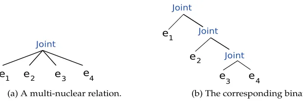
A common assumption made for generating DTs effectively is that they arebinary

trees (Soricut and Marcu 2003; Hernault et al. 2010). That is, multi-nuclear relations (e.g.,

Joint, Same–Unit) involving more than two discourse units are mapped to a hierarchical right-branching binary tree. For example, a flatJoint(e1,e2,e3,e4) (Figure 4a) is mapped to a right-branching binary treeJoint(e1,Joint(e2,Joint(e3,e4))) (Figure 4b).

Figure 4

4.1 Parsing Models

As mentioned before, the job of the intra- and multi-sentential parsing models of CODRA is to assign a probability to each of the constituents of all possible DTs at the sentence level and at the document level, respectively. Formally, given the model parametersΘat a particular parsing scenario (i.e., sentence-level or document-level), for each possible constituentR[i,m,j] in a candidate DT at that parsing scenario, the parsing model estimatesP(R[i,m,j]|Θ), which specifies a joint distribution over the labelRand the structure [i,m,j] of the constituent. For example, when applied to the sentences in Figure 1 separately, the intra-sentential parsing model (with learned parameters Θ_s) estimatesP(R[1, 1, 2]|Θ_s),P(R[2, 2, 3]|Θ_s),P(R[1, 2, 3]|Θ_s), andP(R[1, 1, 3]|Θ_s) for the first sentence, andP(R[4, 4, 5]|Θ_s),P(R[5, 5, 6]|Θ_s),P(R[4, 5, 6]|Θ_s), andP(R[4, 4, 6]|Θ_s) for the second sentence, respectively, for allRranging over the set of relations.

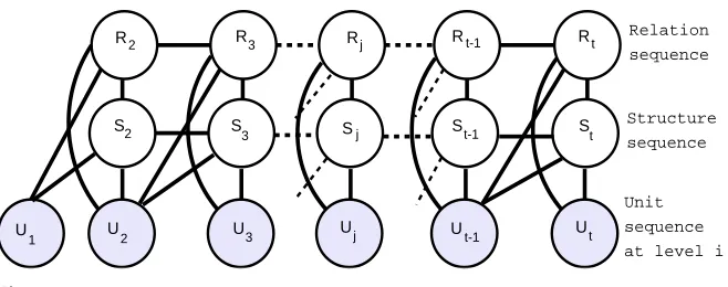
4.1.1 Intra-Sentential Parsing Model.Figure 5 shows the parsing model of CODRA for intra-sentential parsing. The observed nodesUj(at the bottom) in a sequence represent

the discourse units (EDUs or larger units). The first layer of hidden nodes are the struc-ture nodes, whereSj∈ {0, 1}denotes whether two adjacent discourse unitsUj−1andUj

should be connected or not. The second layer of hidden nodes are the relation nodes, withRj∈ {1. . .M}denoting the relation between two adjacent unitsUj−1andUj, where

Mis the total number of relations in the relation set. The connections between adjacent nodes in a hidden layer encode sequential dependencies between the respective hidden nodes, and can enforce constraints such as the fact that a node must have a unique mother, namely, aSj=1 must not follow a Sj−1=1. The connections between the two hidden layers model the structure and the relation of DT constituents jointly.

Notice that the probabilistic graphical model shown in Figure 5 is a chain-structured undirected graphical model (also known asMarkov Random FieldorMRF[Murphy 2012]) with two hidden layers, i.e., structure chain and relation chain. It becomes a Dynamic Conditional Random Field (DCRF)(Sutton, McCallum, and Rohanimanesh 2007) when we directly model the hidden (output) variables by conditioning the clique potentials (i.e., factors) on the observed (input) variables:

P(R2:t,S2:t|x,Θs)= _Z(x,1_Θ s)

t−1

∏

i=2

ϕ(Ri,Ri+1|x,Θs,r)ψ(Si,Si+1|x,Θs,s)ω(Ri,Si|x,Θs,c) (1)

U U U U U

2

2 2

3 j t-1 t

S

S S S S

R R R R R

3

3 j

j t-1

t-1 t

Unit

sequence

at level i Structure

sequence Relation

sequence

U

1

t

Figure 5

where{ϕ}and{ψ}are the factors over the edges of the relation and structure chains, respectively, and{ω}are the factors over the edges connecting the relation and struc-ture nodes (i.e., between-chain edges). Here, x represents input feastruc-tures extracted from the observed variables,Θ_s=[Θ_s,r,Θ_s,s,Θ_s,c] are model parameters, andZ(x,Θ_s) is the partition function. We use the standard log-linear representation of the factors:

ϕ(Ri,Ri+1|x,Θs,r)=exp(ΘTs,rf(Ri,Ri+1, x)) (2) ψ(Si,Si+1|x,Θs,s)=exp(ΘTs,sf(Si,Si+1, x)) (3) ω(Ri,Si|x,Θs,c)=exp(ΘTs,cf(Ri,Si, x)) (4)

wheref(Y,Z, x) is a feature vector derived from the input features x and the local labelsY

andZ, andΘs,yis the corresponding weight vector—that is,Θs,randΘs,sare the weight

vectors for the factors over the relation edges and the structure edges, respectively, and

Θs,cis the weight vector for the factors over the between-chain edges.

A DCRF is a generalization of linear-chain CRFs (Lafferty, McCallum, and Pereira 2001) to represent complex interactions between output variables (i.e., labels), such as when performing multiple labeling tasks on the same sequence. Recently, there has been an explosion of interest in CRFs for solving structured output classification problems, with many successful applications in NLP including syntactic parsing (Finkel, Kleeman, and Manning 2008), syntactic chunking (Sha and Pereira 2003), and discourse chunk-ing (Ghosh et al. 2011) in accordance with the Penn Discourse Treebank (Prasad et al. 2008).

DCRFs, being a discriminative approach to sequence modeling, have several advan-tages over their generative counterparts such asHidden Markov Models (HMMs)and MRFs, which first model the joint distributionp(y, x|Θ), and then infer the conditional distributionp(y|x,Θ). It has been advocated that discriminative models are generally more accurate than generative ones because they do not “waste resources” modeling complex distributions that are observed (i.e.,p(x)); instead, they focus directly on mod-eling what we care about, namely, the distribution of labels given the data (Murphy 2012).

Other key advantages include the ability to incorporate arbitrary overlapping local and global features, and the ability to relax strong independence assumptions. Further-more, CRFs surmount thelabel biasproblem (Lafferty, McCallum, and Pereira 2001) of theMaximum Entropy Markov Model(McCallum, Freitag, and Pereira 2000), which is considered to be a discriminative version of the HMM.

e

1 e2 e

2

2

3

S S₃ R R₃

(a) e 1 e S R 1:2 3 3 3 e e S R 2:3 2:3 (b) 2:3 e 4 S₄ R₄ e 4 S₄ R₄ e 4 S₄ R₄ 1 e e S R 2 2

2 e3:4

S_3:4 R_3:4 1 e S R 1:3 4 4 4 e e S R 2:4 2:4 (c)

2:4 e e

S R 1:2 e 3:4 3:4 3:4 (i) (ii) (iii)

(i) (ii) (iii)

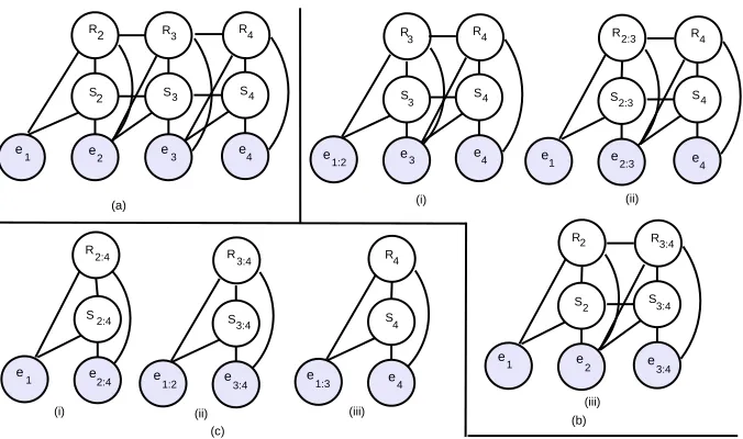
Figure 6

The intra-sentential parsing model is applied to (a) the only possible sequence at the first level, (b) the three possible sequences at the second level, and (c) the three possible sequences at the third level.

P(R3,S3=1|e1,e2,e3,e4,Θs), andP(R4,S4=1|e1,e2,e3,e4,Θs) to obtain the probability of the

DT constituentsR[1, 1, 2],R[2, 2, 3], andR[3, 3, 4], respectively.

At the second level, there are three unit sequences: (e1:2,e3,e4), (e1,e2:3,e4), and (e1,e2,e3:4). Figure 6b shows their corresponding DCRF models. Notice that each of these sequences has a discourse unit that connects two EDUs, and the probability of this con-nection has already been computed at the previous level. CODRA computes the poste-rior marginalsP(R3,S3=1|e1:2,e3,e4,Θs),P(R2:3S2:3=1|e1,e2:3,e4,Θs),P(R4,S4=1|e1,e2:3,e4,Θs),

and P(R3:4,S3:4=1|e1,e2,e3:4,Θs) from these three sequences, which correspond to the

probability of the constituents R[1, 2, 3],R[1, 1, 3],R[2, 3, 4], andR[2, 2, 4], respectively. Similarly, it attains the probability of the constituentsR[1, 1, 4],R[1, 2, 4], andR[1, 3, 4] by computing their respective posterior marginals from the three sequences at the third (i.e., top) level of the candidate DTs (see Figure 6c).

Algorithm 1 describes how CODRA generates the unit sequences at different levels of the candidate DTs for a given number of EDUs in a sentence. Specifically, to compute the probability of a DT constituent R[i,k,j], CODRA generates sequences like (e1,· · ·,ei−1,ei:k,ek+1:j,ej+1,· · ·,en) for 1≤i≤k<j≤n. However,

in doing so, it may generate some duplicate sequences. Clearly, the sequence (e1,· · ·,ei−1,ei:i,ei+1:j,ej+1,· · ·,en) for 1≤i≤k<j<n is already considered for

computing the probability of the constituentR[i+1,j,j+1]. Therefore, it is a duplicate sequence that CODRA excludes from the list of sequences. The algorithm has a complexity ofO(n3), wherenis the number of EDUs in the sentence.

Once CODRA acquires the probability of all possible intra-sentential DT con-stituents, the discourse sub-trees for the sentences are built by applying an optimal parsing algorithm (Section 4.2) using one of the methods described in Section 4.3.

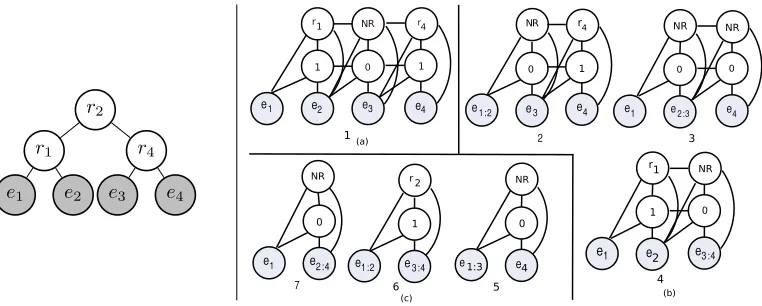
Algorithm 1 is also used to generate sequences for training the model (i.e., learning

Θs). For example, Figure 7 demonstrates how we generate the training instances (right)

Algorithm 1Generating unit sequences for a sentence withnEDUs. Input: Sequence of EDUs: (e1,e2,· · ·,en)

Output: List of sequences:L

fori=1→n−1do // all possible starting positions for the subsequence

forj=i+1→ndo // all possible ending positions for the subsequence

ifj == nthen // sequences at top and bottom levels

fork=i→j−1do // all possible cut points within the subsequence L.append ((e1,· · ·,ei−1,ei:k,ek+1:j,ej+1,· · ·,en))

end

else // sequences at intermediate levels

fork=i+1→j−1do // cut points excluding duplicate sequences L.append ((e1,· · ·,ei−1,ei:k,ek+1:j,ej+1,· · ·,en))

end end end end

generated by the algorithm, we consult the gold DT and see if two discourse units are connected by a relationr (i.e., the corresponding labels are S=1,R=r) or not (i.e., the corresponding labels areS=0,R=NR). We train the model by maximizing the

conditional likelihoodof the labels in each of these training examples (see Equation (1)).

4.1.3 Multi-Sentential Parsing Model. Given the discourse units (sub-trees) for all the individual sentences in a document, a simple approach to build the DT of the document would be to apply a new DCRF model, similar to the one in Figure 5 (with different parameters), to all the possible sequences generated from these units by Algorithm 1 to infer the probability of all possible higher-order (multi-sentential) constituents. How-ever, the number of possible sequences and their length increase with the number of sentences in a document. For example, assuming that each sentence has a well-formed DT, for a document withnsentences, Algorithm 1 generates O(n3) sequences, where

Figure 7

the sequence at the bottom level hasnunits, each of the sequences at the second level hasn-1 units, and so on. Because the DCRF model in Figure 5 has a “fat” chain struc-ture, one could use the forward–backward algorithm for exact inference in this model (Murphy 2012). Forward–backward on a sequence containing T units costs O(TM2) time, where M is the number of relations in our relation set. This makes the chain-structured DCRF model impractical for multi-sentential parsing of long documents, since learning requires running inference on every training sequence with an overall time complexity ofO(TM2_n3_)=O(M2_n4_{) per document (Sutton and McCallum 2012).}

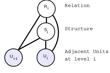
To address this problem, we have developed a simplified parsing model for multi-sentential parsing. Our model is shown in Figure 8. The two observed nodes Ut−1 andUtare two adjacent (multi-sentential) discourse units. The (hidden) structure node

S∈ {0, 1}denotes whether the two discourse units should be linked or not. The other hidden nodeR∈ {1. . .M}represents the relation between the two units. Notice that similar to the model in Figure 5, this is also an undirected graphical model and becomes a CRF model if we directly model the labels by conditioning the clique potentialϕon the input features x, derived from the observed variables:

P(Rt,St|x,Θd)= _Z(x,1_Θ d)

ϕ(Rt,St|x,Θd) (5)

ϕ(Rt,St|x,Θd)=exp(ΘTd f(Rt,St, x)) (6)

wheref(Rt,St, x) is a feature vector derived from the input features x and the labelsRt

and St, and Θd is the corresponding weight vector. Although this model is similar in

spirit to the parsing model in Figure 5, it now breaks the chain structure, which makes the inference much faster (i.e., a complexity ofO(M2)). Breaking the chain structure also allows CODRA to balance the data for training (an equal number of instances withS=1 andS=0), which dramatically reduces the learning time of the model.

CODRA applies this parsing model to all possible adjacent units at all levels in the multi-sentential case, and computes the posterior marginals of the relation– structure pairsP(Rt,St=1|Ut−1,Ut,Θd) using the forward–backward algorithm to obtain

the probability of all possible DT constituents. Given the sentence-level discourse units, Algorithm 2, which is a simplified variation of Algorithm 1, extracts all possible adjacent discourse units for multi-sentential parsing. Similar to Algorithm 1, Algorithm 2 also has a complexity ofO(n3_{), wherenis the number of sentence-level discourse units.}

U U

t-1 t

S R_t

Adjacent Units

at level i Structure Relation

t

Figure 8

Algorithm 2Generating all possible adjacent discourse units at all levels of a document-level discourse tree.

Input: Sequence of units: (U1,U2,· · ·Un), where Ux[0]:= start EDU ID of unitx, and

Ux[1]:=end EDU ID of unitx.

Output: List of adjacent units:L

fori=1→n−1do // all possible starting positions for the subsequence

forj=i+1→ndo // all possible ending positions for the subsequence

fork=i→j−1do // all possible cut points within the subsequence Left=Ui[0] :Uk[1]

Right=Uk+1[0] :Uj[1]

L.append ((Left,Right)) end

end end

Both our intra- and multi-sentential parsing models are designed using MALLET’s graphical model toolkit GRMM (McCallum 2002). In order to avoid overfitting, we regularize the CRF models withl2regularization and learn the model parameters using the limited-memory BFGS (L-BFGS) fitting algorithm.

4.1.4 Features Used in the Parsing Models. Crucial to parsing performance is the set of features used in the parsing models, as summarized in Table 1. We categorize the features into seven groups and specify which groups are used in what parsing model. Notice that some of the features are used in both models. Most of the features have been explored in previous studies (e.g., Soricut and Marcu 2003; Sporleder and Lapata 2005; Hernault et al. 2010). However, we improve some of these as explained subsequently.

The features are extracted from two adjacent discourse unitsUt−1andUt.

Organiza-tionalfeatures encode useful information about text organization as shown by duVerle and Prendinger (2009). We measure the length of the discourse units as the number of

EDUsandtokensin it. However, in order to better adjust to the length variations, rather than computing their absolute numbers in a unit, we choose to measure theirrelative numberswith respect to their total numbers in the two units. For example, if the two discourse units under consideration contain three EDUs in total, a unit containing two of the EDUs will have a relative EDU number of 0.67. We also measure thedistancesof the units in terms of the number of EDUs from the beginning and end of the sentence (or text in the multi-sentential case). Text structural features capture the correlation between text structure and rhetorical structure by counting the number ofsentenceand

paragraphboundaries in the discourse units.

Discourse cues (e.g.,because, but), when present, signal rhetorical relations between two text segments, and have been used as a primary source of information in earlier studies (Knott and Dale 1994; Marcu 2000a). However, recent studies (Hernault et al. 2010; Biran and Rambow 2011) suggest that an empirically acquiredlexical N-gram dictionary is more effective than a fixed list of cue phrases, since this approach is domain independent and capable of capturing non-lexical cues such as punctuation.

Table 1

Features used in our intra- and multi-sentential parsing models.

8 Organizational features Intra & Multi-Sentential

Number of EDUs inunit 1(orunit 2). Number of tokens inunit 1(orunit 2).

Distance of unit 1 in EDUs to thebeginning(or to theend). Distance of unit 2 in EDUs to thebeginning(or to theend).

4 Text structural features Multi-Sentential

Number of sentences inunit 1(orunit 2). Number of paragraphs inunit 1(orunit 2).

8 N-gram featuresN∈{1, 2, 3} Intra & Multi-Sentential

Beginning(orend) lexical N-grams in unit 1. Beginning(orend) lexical N-grams in unit 2. Beginning(orend) POS N-grams in unit 1. Beginning(orend) POS N-grams in unit 2.

5 Dominance set features Intra-Sentential

Syntactic labels of theheadnode and theattachmentnode. Lexical heads of theheadnode and theattachmentnode. Dominance relationshipbetween the two units.

9 Lexical chain features Multi-Sentential

Number of chains spanning unit 1 and unit 2. Number of chains start in unit 1 and end in unit 2. Number of chainsstart(orend) inunit 1(or inunit 2). Number of chains skipping both unit 1 and unit 2. Number of chains skippingunit 1(orunit 2).

2 Contextual features Intra & Multi-Sentential

Previousandnextfeature vectors.

2 Sub-structural features Intra & Multi-Sentential

Root nodes of theleftandrightrhetorical sub-trees.

More specifically, given an N-gramx, we compute itsconditional entropy Hwith respect toSandRas follows:8

H(S,R|x)=− ∑

s∈S r∈R

logc(x,s,r)

c(x) (7)

wherec(x) is the empirical count of N-gramx, andc(x,s,r) is the joint empirical count of N-gramxwith the labelssandr. This is in contrast to HILDA (Hernault et al. 2010), which ranks the N-grams by their frequencies in the training corpus. However, Blitzer

(2008) found mutual information to be more effective than frequency as a method for feature selection. Intuitively, the most informative discourse cues are not only the most frequent, but also the ones that are indicative of the labels in the training data. In addition to the lexical N-grams we also encode thePOS tags of the first and last N

tokens (N∈{1, 2, 3}) in a discourse unit as shallow-syntactic features in our models.

Figure 9

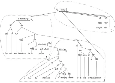
Lexico-syntactic featuresdominance setsextracted from the Discourse Segmented Lexicalized Syntactic Tree (DS-LST) of a sentence have been shown to be extremely effective for intra-sentential discourse parsing in SPADE (Soricut and Marcu 2003). Figure 9a shows the DS-LST (i.e., lexicalized syntactic tree with EDUs identified) for a sentence with three EDUs from the RST–DT corpus, and Figure 9b shows the corre-sponding discourse tree. In a DS-LST, each EDU except the one with the root node must have a head node NH that is attached to an attachment node NA residing in a separate

EDU. A dominance setD(shown at the bottom of Figure 9a) contains theseattachment

points (shown in boxes) of the EDUs in a DS-LST. In addition to the syntactic and lexical information of the head and attachment nodes, each element in the dominance set also includes a dominance relationship between the EDUs involved; the EDU with the attachment node dominates (represented by “>”) the EDU with the head node.

Soricut and Marcu (2003) hypothesize that the dominance set (i.e., lexical heads, syntactic labels, and dominance relationships) carries the most informative clues for intra-sentential parsing. For instance, the dominance relationship between the EDUs in our example sentence is 3>1>2, which favors the DT structure [1, 1, 2] over [2, 2, 3]. In order to extract dominance set features for two adjacent discourse unitsUt−1andUt,

containing EDUsei:jandej+1:k, respectively, we first compute the dominance set from

the DS-LST of the sentence. We then extract the element from the set that holds across the EDUs j and j+1. In our example, for the two units, containing EDUs e1 and e2, respectively, the relevant dominance set element is(1, efforts/NP)>(2, to/S). We encode the syntactic labels and lexical heads ofNHandNA, and the dominance relationship as

features in our intra-sentential parsing model.

Lexical chains(Morris and Hirst 1991) are sequences of semantically related words that can indicate topical boundaries in a text (Galley et al. 2003; Joty, Carenini, and Ng 2013). Features extracted from lexical chains are also shown to be useful for finding paragraph-level discourse structure (Sporleder and Lapata 2004). For example, consider the text with four paragraphs (P1toP4) in Figure 10a. Now, let us assume that there is a lexical chain that spans the whole text, skipping paragraphsP2 andP3, while a second chain only spansP2andP3. This situation makes it more likely thatP2andP3should be linked in the DT before either of them is linked with another paragraph. Therefore, the DT structure in Figure 10b should be more likely than the structure in Figure 10c.

One challenge in computing lexical chains is that words can have multiple senses, and semantic relationships depend on the sense rather than the word itself. Several methods have been proposed to compute lexical chains (Barzilay and Elhadad 1997; Hirst and St. Onge 1997; Silber and McCoy 2002; Galley and McKeown 2003). We follow the state-of-the-art approach proposed by Galley and McKeown (2003), which extracts lexical chains after performing Word Sense Disambiguation (WSD).

P₁ P₂ P P

3 4 P1 P2 P3 P4 P1 P2 P3 P4

(a) (b) (c)

Figure 10

bank

company

institution

riverside bank

R R

H H

H H

H

H

S

bank

company

institution

riverside bank

(bank, company, institution, bank)

(riverside)

(a)

(b)

Figure 11

Extracting lexical chains. (a) A Lexical Semantic Relatedness Graph (LSRG) for five noun-tokens. (b) Resultant graph after performing WSD. The box at the bottom shows the lexical chains.

In the preprocessing step, we extract the nouns from the document and lemmatize them using WordNet’s built-inmorphyfunction (Fellbaum 1998). Then, by looking up in WordNet we expand each noun to all of its senses, and build a Lexical Semantic Relatedness Graph (LSRG) (Galley and McKeown 2003; Chali and Joty 2007). In an LSRG, the nodes represent noun-tokens with their candidate senses, and the weighted edges between senses of two different tokens represent one of the three semantic rela-tions:repetition, synonym, andhypernym. For example, Figure 11a shows a partial LSRG, where the tokenbankhas two possible senses, namely,money bankandriver bank. Using themoney bank sense, bank is connected with institutionand company by hypernymy relations (edges marked withH), and with anotherbankby a repetition relation (edges marked withR). Similarly, using theriver banksense, it is connected withriversideby a hypernymy relation and withbankby a repetition relation. Nouns that are not found in WordNet are considered as proper nouns having only one sense, and are connected by onlyrepetitionrelations.

We use this LSRG first to perform WSD, then to construct lexical chains. For WSD, the weights of all edges leaving the nodes under their different senses are summed up and the one with the highest score is considered to be the right sense for the word-token. For example, if repetition and synonymy are weighted equally, and hypernymy is given half as much weight as either of them, the score ofbank’s two senses are: 1+0.5+

0.5=2 for the sensemoney bankand 1+0.5=1.5 for the senseriver bank. Therefore, the selected sense forbank in this context isriver bank. In case of a tie, we select the sense that is most frequent (i.e., the first sense in WordNet). Note that this approach to WSD is different from that of Sporleder and Lapata (2004), which takes a greedy approach.

We also consider more contextual information by including the above features computed for the neighboring adjacent discourse unit pairs in the current feature vector. For example, the contextual features for unitsUt−1 andUtinclude the feature vector

computed fromUt−2andUt−1and the feature vector computed fromUtandUt+1. We incorporatehierarchical dependenciesbetween the constituents in a DT by rhetor-icalsub-structuralfeatures. For two adjacent unitsUt−1andUt, we extract the roots of

the two rhetorical sub-trees. For example, the root of the rhetorical sub-tree spanning over EDUs e1:2 in Figure 9b is Elaboration–NS. However, extraction of these features assumes the presence of labels for the sub-trees, which is not the case when we apply the parser to a new text (sentence or document) in order to build its DT in a non-greedy fashion. One way to deal with this is to loop twice through the parsing process using two different parsing models—one trained with the complete feature set, and the other trained without the sub-structural features. We first build an initial, sub-optimal DT using the parsing model that is trained without the sub-structural features. This intermediate DT will now provide labels for the sub-structures. Next we can build a final, more accurate DT by using the complete parsing model. This idea of two-pass discourse parsing, where the second two-pass performs post-editingusing additional features, has recently been adopted by Feng and Hirst (2014) in their greedy parser.

One could even continue doing post-editing multiple times until the DT converges. However, this could be very time consuming as each post-editing pass requires: (1) ap-plying the parsing model to every possible unit sequence and computing the posterior marginals for all possible DT constituents, and (2) using the parsing algorithm to find the most probable DT. Recall from our earlier discussion in Section 4.1.3 that for n

discourse units andMrhetorical relations, the first step requiresO(M2_n4_{) andO(M}2_n3₎ for intra- and multi-sentential parsing, respectively; we will see in the next section that the second step requiresO(Mn3). In spite of the computational cost, the gain we attained in the subsequent passes was not significant for our development set. Therefore, we restrict our parser to only one-pass post-editing.

Note that in parsing models where the score (i.e., likelihood) of a parse tree de-composes across local factors (e.g., the CRF-based syntactic parser of Finkel, Kleeman, and Manning [2008]), it is possible to define asemiringusing the factors and the local scores (e.g., given by the inside algorithm). The CKY algorithm could then give the optimal parse tree in a single post-editing pass (Smith 2011). However, because our intra-sentential parsing model is designed to capture sequential dependencies between DT constituents, the score of a DT does not directly decompose across factors over discourse productions. Therefore, designing such a semiring was not possible in our case.

In addition to these features, we also experimented with other features including

WordNet-based lexical semantics,subjectivity, andTF.IDF-based cosine similarity. However, because such features did not improve parsing performance on our development set, they were excluded from our final set of features.

4.2 Parsing Algorithm

describe the specific case of generating the single most probable DT, then we describe how to generalize this algorithm to produce thekmost probable DTs for a given text.

Formally, the search problem for finding the most probable DT can be written as

DT∗=argmax

DT

P(DT|Θ) (8)

whereΘspecifies the parameters of the parsing model (intra- or multi-sentential). Given

ndiscourse units, our parsing algorithm uses the upper-triangular portion of then×n

dynamic programming tableD, where cellD[i,j] (fori<j) stores:

D[i,j]=P(r∗[Ui(0),Um∗(1),Uj(1)]) (9)

whereUx(0) andUx(1) are the start and end EDU Ids of discourse unitUx, and

(m∗,r∗)= argmax

i≤m<j;R∈{1···M}

P(R[Ui(0),Um(1),Uj(1)])×D[i,m]×D[m+1,j] (10)

Recall that the notation R[Ui(0),Um(1),Uj(1)] in this expression refers to a rhetorical

relationRthat holds between the discourse unit containing EDUsUi(0) throughUm(1)

and the unit containing EDUsUm(1)+1 throughUj(1).

In addition toD, which stores theprobabilityof the most probable constituents of a DT, the algorithm also simultaneously maintains two othern×ndynamic programming tablesS andR for storing the structure (i.e.,Um∗(1)) and the relations (i.e.,r∗) of the

corresponding DT constituents, respectively. For example, given four EDUse1· · ·e4, the Sand Rdynamic programming tables at the left side in Figure 12 together represent the DT shown at the right. More specifically, to find the DT, we first look at the top-right entries in the two tables, and findS[1, 4]=2 andR[1, 4]=r2, which specify that the two discourse unitse1:2ande3:4should be connected by the relationr2 (the root in the DT). Then, we see how EDUse1ande2should be connected by looking at the entriesS[1, 2] andR[1, 2], and findS[1, 2]=1 andR[1, 2]=r1, which indicates that these two units should be connected by the relationr1 (the left pre-terminal in the DT). Finally, to see how EDUse3ande4should be linked, we look at the entriesS[3, 4] andR[3, 4], which tell us that they should be linked by the relationr4(the right pre-terminal). The algorithm

Figure 12

works in polynomial time. Specifically, forndiscourse units andMnumber of relations, the time and space complexities areO(n3M) andO(n2), respectively.

A key advantage of using a probabilistic parsing algorithm like the one we use is that it allows us to generate a list ofkmost probable parse trees. It is straightforward to generalize the above algorithm to produce kmost probable DTs. Specifically, when filling up the dynamic programming tables, rather than storing a single best parse for each sub-tree, we store and keep track (i.e., using back-pointers) ofk-best candidates simultaneously. One can show that the time and space complexities of thek-best version of the algorithm areO(n3_Mk2_{logk) andO(k}2_{n), respectively (Huang and Chiang 2005).} Note that, in contrast to other document-level discourse parsers (Marcu 2000b; Subba and Di-Eugenio 2009; Hernault et al. 2010; Feng and Hirst 2012, 2014), which use a greedy algorithm, CODRA finds a discourse tree that is globally optimal.9 _This approach of CODRA is also different from the sentence-level discourse parser SPADE (Soricut and Marcu 2003). SPADE first finds thetree structurethat is globally optimal, then it assigns the most probablerelationsto the internal nodes. More specifically, the cellD[i,j] in SPADE’s dynamic programming table stores

D[i,j]=P([Ui(0),Um∗(1),Uj(1)]) (11)

where m∗=argmax

i≤m<j

P([Ui(0),Um(1),Uj(1)]). Disregarding the relation label R while

populatingD, this approach may find a discourse tree that is not globally optimal.

4.3 Document-Level Parsing Approaches

Now that we have presented our intra-sentential and multi-sentential parsing com-ponents, we are ready to describe how they can be effectively combined in a uni-fied framework (Figure 2) to perform document-level rhetorical analysis. Recall that a key motivation for a two-stage10 _{parsing is that it allows us to capture the strong} correlation between text structure and discourse structure in a scalable, modular, and flexible way. In the following, we describe two different approaches to model this correlation.

4.3.1 1S–1S (1 Sentence–1 Sub-tree). A key finding from previous studies on sentence-level discourse analysis is that most sentences have a well-formed discourse sub-tree in the full document-level DT (Soricut and Marcu 2003; Fisher and Roark 2007). For example, Figure 13a shows 10 EDUs in three sentences (see boxes), where the DTs for the sentences obey their respective sentence boundaries.

Our first approach, called 1S–1S (1 Sentence–1 Sub-tree), aims to maximally exploit this finding. It first constructs a DT for every sentence using our intra-sentential parser, and then it provides our multi-sentential parser with the sentence-level DTs to build the rhetorical parse for the whole document.

4.3.2 Sliding Window. Although the assumption made by 1S–1S clearly simplifies the parsing process, it completely ignores the cases where rhetorical structures violate

9 We agree that with potentially sub-optimal, sub-structural features in the parsing model, CKY may end up finding a sub-optimal DT. But that is a separate issue.