A Graph Theoretic Framework for Semantic Distance

Semantic Distance

Vivian Tsang

Suzanne Stevenson

Many NLP applications entail that texts are classified based on their semantic distance (how similar or different the texts are). For example, comparing the text of a new document to that of documents of known topics can help identify the topic of the new text. Typically, a distributional distance is used to capture the implicit semantic distance between two pieces of text. However, such approaches do not take into account the semantic relations between words. In this article, we introduce an alternative method of measuring the semantic distance between texts that integrates distributional information and ontological knowledge within a network flow formalism. We first represent each text as a collection of frequency-weighted concepts within an ontology. We then make use of a network flow method which provides an efficient way of explicitly measuring the frequency-weighted ontological distance between the concepts across two texts. We evaluate our method in a variety of NLP tasks, and find that it performs well on two of three tasks. We develop a new measure of semantic coherence that enables us to account for the performance difference across the three data sets, shedding light on the properties of a data set that lends itself well to our method.

1. Introduction

Many natural language tasks can be cast as a problem of comparing texts in terms of their semantic distance. For example, given a suitable text distance measure, document classification can be performed by comparing the text of a new document to the text of various documents whose topics are known. The new document is then labelled with the topic of the document whose text is most similar to it. In general, the texts to be compared may be full documents, as in this example, or may be portions of documents, or even collections of documents. Using text comparison to perform semantic classifi-cation has been adopted in a variety of natural language processing (NLP) tasks, from document classification (Scott and Matwin 1998; Rennie 2001; Al-Mubaid and Umair 2006), to prepositional phrase attachment (Pantel and Lin 2000), to spelling correction (Budanitsky and Hirst 2001).

∗Department of Computer Science, University of Toronto, 6 King’s College Road, Toronto, Ontario M5S 3G4, Canada. E-mail: [email protected].

∗∗Department of Computer Science, University of Toronto, 6 King’s College Road, Toronto, Ontario M5S 3G4, Canada. E-mail: [email protected].

Distributional methods for semantic distance are widely used and highly successful in comparing texts that are represented as bags of words with associated frequencies of occurrence (Lee 2001; Weeds, Weir, and McCarthy 2004; Pedersen, Banerjee, and Patwardhan 2005). In document classification, for example, the text of a document may be represented as a word frequency vector, which is compared using a distributional distance measure to each of the word frequency vectors of the texts of the documents of known topics. In this way, distributional distance between word vectors captures the semantic distance between two texts that is implicitly encoded in the set of words used in each.

Semantic distance can also be measured more explicitly, by using the relations in an ontology as the direct encoding of semantic association. However, such approaches have generally been limited to calculating the distance between two individual con-cepts, rather than capturing the distance between twosets of concepts corresponding to two texts. Numerous measures have been proposed, for example, for capturing the distance between two concepts in WordNet, typically relying on the synonymy (synset) and hyponymy (is-a) relations (Wu and Palmer 1994; Resnik 1995; Jiang and Conrath 1997, among others). Using such an ontological measure to compare two texts (collections of words instead of single words) might involve mapping each word of a text to its appropriate concept(s) in the ontology, and then calculating the aggregate distance between the two resulting sets of concepts across the ontological relations. For example, one might calculate the semantic distance between the two texts as the average, minimum, maximum, or summed ontological distance between the individual elements of the two sets of concepts (Corley and Mihalcea 2005).

Observe that each of these approaches to text comparison—distributional and ontological—encodes information not contained in the other. Distributional distance captures important information about frequency of occurrence of the words that consti-tute the target text, whereas ontological distance captures essential semantic knowledge that has been encoded in the relations of an ontology. In response, previous work has attempted to combine distributional and ontological information in computing seman-tic distance. For example, researchers have developed measures of semanseman-tic distance between texts that apply distributional distances to concept vectors of frequencies rather than to word vectors (McCarthy 2000; Mohammad and Hirst 2006). However, these ap-proaches only make pairwise comparisions between the elements of the concept vectors, and do not take into account the important ontological relations among the concepts. In order to capture such relations, other methods have instead integrated distributional information into an ontological method. However, such approaches have heretofore been limited to measuring distance between two individual concepts. For example, some ontological measures use corpus frequencies of words to yield concept weights that are taken into account in measuring the distance between two concepts (Resnik 1995; Jiang and Conrath 1997). What has been missing is an approach to semantic distance between two texts—two sets of words—that can truly integrate distributional and ontological (relational) information, drawing more fully on their complementary advantages for text comparison.

By exploiting the relational structure of the ontology, we can explicitly measure the ontological distance over the paths between two profiles. Using the frequencies on the concept nodes, we weight these paths according to the frequency distribution of words in the two texts. The resulting calculation yields a frequency-weighted ontological distance between the two sets of concepts. Thus, we view a text not as a set of items to be compared individually to those in another set (with those individual distances then somehow combined, e.g., as in Corley and Mihalcea [2005]), but rather as a distribution of “mass” within a graph that encodes the semantic relations across the two sets, and use a weighted graph-based approach that captures the aggregate distance between the two frequency masses.

To our knowledge, this is the first method to integrate ontological and distributional information in the graphical calculation of text distance. This article describes the use of the new measure in several different types of NLP text comparison tasks, in order to explore the situations in which such an approach can be effective. Given the novelty of the approach, the task-based evaluation is not intended as the last word on the usefulness of the method, but rather as a first suite of experiments across different types of text comparison tasks to illuminate some of the strengths and weaknesses of such an approach to text distance. We thus analyze the results in detail to identify future directions for further illuminating when and to what extent the method might be useful. The analysis reveals that our method is not consistently successful across our sample tasks. We hypothesize that, because ontological relations play an integral role in our semantic distance measure, the measure is less effective when the semantic profile for a text (the set of corresponding concepts) lacks semantic coherence. Other work has explored ways to measure the semantic coherence of a set of concepts in terms of their connectedness within an ontology (Gurevych et al. 2003). Because a semantic profile in our work includes both ontological (relational) and distributional (frequency) knowledge, we require a measure of semantic coherence that takes both into account. We develop a novel measure of semantic coherence called profile density that captures both the ontological and distributional coherence of a set of frequency-weighted concepts, and apply it to the data sets used in the different tasks to better understand the performance of our semantic distance measure.

Our distance measure is cast as a graphical text comparison task within a network flow framework as described in Section 2. In Section 3, we give an overview of our exploration of the method on three types of text comparison problems. The following three sections present experimental results and analysis of applying our method to the various tasks: verb alternation detection (Section 4), name disambiguation (Section 5), and document classification (Section 6). In Section 7, we describe our profile density measure and use it to analyze the properties of the data sets that lead to the performance differential across the tasks. We conclude the paper with a description of related work in text comparison and graph-theoretic NLP approaches (Section 8) and a discussion of some future directions for our research (Section 9).

2. The Network Flow Method

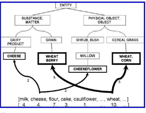
As noted previously, we treat an ontology as a graph and represent a text as a semantic profile—a collection of nodes in the graph (concepts in the ontology), each having a weight (its frequency). For example, in Figure 1, a small text consisting of the words

Figure 1

A small text represented as a collection of weighted nodes in a fragment of WordNet.

larger graph (with the thickness of the boxes in the figure indicating weight), and two such weighted subgraphs are connected via a set of paths in the graph.

Our goal is to measure the distance between two subgraphs (representing two texts to be compared), taking into account both the ontological distance between the component concepts and their frequency distributions. To achieve this, we measure the amount of “effort” required to transform one profile to match the other graphically: The more similar they are, the less effort it takes to transform one into the other. (This view is similar to that motivating the use of “earth mover’s distance” in computer vision [Levina and Bickel 2001].) In Section 2.1, we first give the intuitive motivation for the approach in terms of the properties of semantic distance that we want to cap-ture by considering transport effort. We then present the mathematical formulation of our graph-based method as a minimum cost flow (MCF) problem in Section 2.2, and describe the formulation of our task within this network flow framework in Section 2.3. In Section 2.4, we return to the properties we identify in Section 2.1 to explain how they are reflected in the MCF formulation.

2.1 An Intuitive Overview

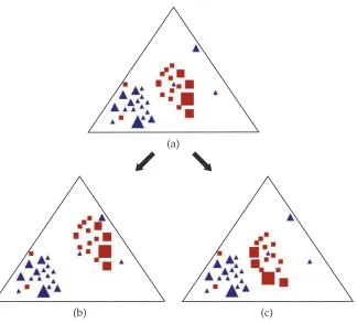
Figure 2

Two subgraphs (one represented by squares, the other, triangles) with varying degrees of overlap and, therefore, similarity within an ontology. Figure (b) differs from Figure (a) in terms of the ontological distance between the square and the triangle clusters. Figure (c) differs from Figure (a) in terms of the size of the individual squares.

The transport effort is determined by both the amount of mass to move and the graphical distance over which it must travel. First consider graphical (ontological) distance between the profiles. Assume the calculated distance between the two profiles in Figure 2(a) is d. In Figure 2(b), the triangle profile is exactly the same. By contrast, although the square profile has the same internal properties (same frequency distribu-tion and graphical structure), its locadistribu-tion is further from the triangles. Because the two profiles occupy more distant portions of the ontological space, they are less semantically similar than in Figure 2(a). As desired, the extra ontological distance over which the square frequency mass must be transported to the triangles will cause the calculated distance in Figure 2(b) to be larger thand.

It is worth noting explicitly that this notion of semantic distance as transport effort of concept frequency over the relations (edges) of an ontology differs significantly from an approach to semantic distance that utilizes concept vectors of frequency. By crucially utilizing the relations between concepts in calculating semantic distance, our approach can determine the distance between texts that use related but non-equivalent concepts. For example, our measure will find greater similarity between a text that discusses milkand one that discussescheesethan between one that discusses milkand one that discussesbread. A vector distance would find each of these equally dissimilar, because there are no concepts in common, and there is no way to relatemilktocheese.1

The intuitive examples in Figure 2 show that calculating semantic distance as transport effort captures in a well-motivated way both the ontological distance between the profiles and their weighting by the distributional amounts of the concept nodes. In the next subsection, we describe a mathematical formulation that captures the relevant properties of our problem in a network flow framework. Network flow methods are often used in computer science for modelling such transport effort, for example, in communication or transportation networks.

2.2 Minimum Cost Flow

Our intuitive transport effort examples above can be viewed as a supply–demand problem, in which we find the minimum cost flow (MCF) from the supply profile to the demand profile to meet the requirements of the latter. Mathematically, letG=(N,E) be a connected graph representing an ontology, whereNis the set of nodes representing the individual concepts, andE is the set of edges representing the relations between the concepts. (Most ontologies are connected; in the case of a forest, adding an arbi-trary root node yields a connected graph.) Each edge has a cost c:E→R, which is the ontological distance of the edge. Each node i∈N is associated with a value b(i) such that b:N→R indicates its available supply (b(i)>0), its demand (b(i)<0), or neither (b(i)=0). The goal is to find a flow from supply nodes to demand nodes that satisfies the supply/demand constraints of each node and minimizes the overall “trans-port cost.”

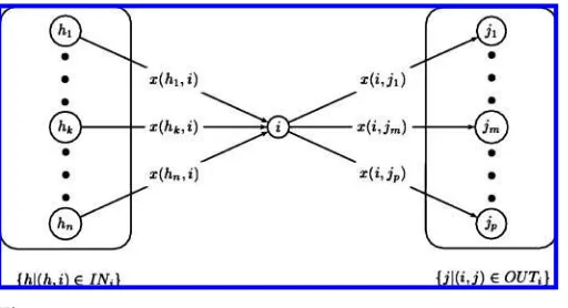
First, we have to define a function to describe the flow enteringivia an incoming edge (h,i) and exiting i via an outgoing edge (i,j). Let IN_i be the set of edges (h,i) with a flow entering node i; similarly, let OUTi be the set of edges (i,j) with a flow exiting nodei. Then, the flow entering and exiting nodeiis captured byx:E→Rsuch that we can observe the combined incoming flow, _(h,i)∈IN

ix(h,i), from the entering edgesINi, as well as the combined outgoing flow,

(i,j)∈OUTix(i,j), via the exiting edges OUT_i (see Figure 3). A valid flow, x, must be found such that the net flow at each node—the difference between its exiting flow and its entering flow—equals its specified supply or demand constraints. For example, in Figure 2 where the squares represent the supply and the triangles represent the demand, a solution forxwould allow us to transport all the weight at the squares to fill the triangles, via a set of routes connecting them.

Figure 3

An illustration of flow entering and exiting nodei.

Formally, the MCF problem can be stated as follows (from Chv ´atal 1983):

Minimize z(x)=

(i,j)∈E

c(i,j)·x(i,j) (1)

subject to

(i,j)∈OUTi

x(i,j)−

(h,i)∈INi

x(h,i)=b(i),∀i∈N (2)

and x(i,j)≥0,∀(i,j)∈E (3)

The constraint specified by Equation (2) ensures that the difference between the flow entering and exiting each node imatches its supply or demand b(i) exactly. The next constraint, Equation (3), ensures that the flow is transported from the supply to the demand but not in the opposite direction. The calculation ofzin Equation (1) (which is subject to these constraints) multiplies the amount of flow travelling along each edge, x(i,j), by the transportation cost of using that edge,c(i,j). Taking the summation over all edges of the productc(i,j)·x(i,j) yields the desired transport effort of using the supply to fill the demand.2

2.3 Semantic Distance as MCF

To cast our text comparison task into this framework, we first represent each text as a semantic profile in an ontology. The profile of one text is chosen as the supply (S) and the other as the demand (D); our distance measure is symmetric, so this choice is arbitrary. In our examples in Section 2.1, the square profile was seen as the supply and the triangle

profile as the demand. The concept frequencies of the profiles are normalized, so that the total supply equals the total demand.

The cost of the routes between nodes is determined by a semantic distance measure defined over the nodes in the ontology—that is, a measure of individual concept-to-concept distance. A relation (such as hyponymy) between two concepts iand j is represented by an edge (i,j), and the cost c on the edge (i,j) can be defined as the concept-to-concept distance betweeniandj. For simplicity in this article, we use edge distance as our concept-to-concept distance measurec; that is, each edge (i,j) has a cost of 1, and the distance between any two concepts is the number of edges separating them.3

Next, we must determine the value ofb(i) at each concept nodei. In the simple case,ioccurs in only one profile or the other. Ifi∈S,b(i) is set to the normalized sup-ply frequency, fS(i). If i∈D, b(i) is set to the negative of the normalized demand frequency,−fD(i), since demand is indicated by a value less than zero. However,imay be part of both the supply and demand profiles, and then b(i) must be set to the net supply/demand at nodei. Thus we have:

b(i)=f_S(i)−f_D(i) (4)

For example, if the supply profile contains a nodecarwith frequency of 0.25, and the same node in the demand profile has a frequency of 0.7, thenb(car) is−0.45. In other words, the nodecarhas a net demand of 0.45.

Recall that our goal is to transport all the supply to meet the demand; the key step is to determine the optimal routes between Sand Dsuch that the constraints in Equation (2) and Equation (3) are satisfied. The total distance of the routes, or the MCF— z(x) in Equation (1)—is the distance between the two semantic profiles.

2.4 Ontological and Distributional Factors in MCF

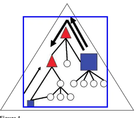
To see how the factors of ontological distance and frequency distribution play out in the MCF formulation, let’s return to our square and triangle profile example. Consider a hypothetical zoomed-in area of the earlier diagram in Figure 2(a), shown in Figure 4. Here we assume that the square nodes have a net supply (b(i)>0) and the triangle nodes have a net demand (b(i)<0).4 The size of the square and triangle nodes in the figure indicates |b(i)|—i.e., the relative supply/demand, respectively. The circles indicate nodes with neither supply nor demand constraints—i.e.,b(i)=0. Each arrow from nodeito nodejindicates the source and destination for transported flow from a square node to a triangle. The length of an arrow represents the ontological distance, c(i,j), and the width indicates the amount of flow, x(i,j). Note that the mass at the rightmost square in the figure has to be distributed over the two triangles, and the mass at the leftmost square is transported over a path with one edge (as indicated by

3 Some semantic distances, such as those of Lin (1998) and Resnik (1995), do not directly use the underlying graph structure of the ontology in calculating the distance between two concepts. Using this type of distance in our MCF framework requires an extra graph transformation step; see Tsang and Stevenson (2006) for more details.

4 Earlier we made the simplifying assumption that square nodes were the supply profile and triangle nodes the demand profile. We have now seen that a node can belong to both profiles, and its

Figure 4

An example of transporting the weights at the square nodes (supply nodes) to the triangle nodes (demand nodes). The circle nodes have zero supply/demand requirement.

the arrow nearby) instead of a path with three edges (with two circle nodes on the path). The aggregated length and width of the three arrows corresponds to the minimum cost flow, i.e., the semantic distance between the profiles represented by the squares and triangles.

Both the ontological distance between nodes and the node weights are important in determining the minimum cost flow. The role of ontological information in the MCF formulation is clear. If the squares were further away from the triangles in the ontology in Figure 4—that is, if more edges separated the squares and the triangles—the sets of concepts they represent would be less semantically similar. The length of the arrows (representingc(i,j)) would be greater, and the resulting MCF would be larger, reflecting the greater semantic distance between the profiles. Distributional information in this method is equally critical to the distance calculation, because it determines the amount of supply/demand at each node. If the squares in Figure 4 were more uniformly sized, the two profiles would be more semantically similar because the weight would be distributed more similarly across the ontological space. In this case, less flow would have to travel from the rightmost square to the leftmost triangle (i.e., the corresponding arrow would be thinner, representingx(i,j)), and the resulting MCF would therefore be smaller. In short, our MCF method captures the desired property that both ontological distance between profile nodes and their frequency distributions determine the overall semantic distance between two profiles.

3. Evaluation: Experimental Tasks and Methodology

underlying argument structure. The task is achieved by comparing the set of head words that occur with the verb in each of two different syntactic positions (e.g., subject of intransitive and object of transitive). In this task, the words that make up the texts to be compared have a particular syntactic relation to the verb under consideration. In proper name disambiguation (Section 5), we classify the sense of an ambiguous name according to its local context. This task is similar to word sense disambiguation (WSD), in picking the intended sense of a term, but also has similarities to topic identification, since the proper name delineates a particular domain of discourse. In this task, we compare the text constituting the ambiguous instance to texts representing each of the known referents of the name. Here, the words of a text are extracted from a small window of occurrence around the target name token (25 words on each side), regardless of the syntactic relations among the words. For the known referents, the words from these windows are aggregated across a small set of labelled instances. In document classification (Section 6), a text is classified into one of a restricted number of topic categories. The text to be classified consists of all the words in a document; for each topic, it is compared to a set of words corresponding to a small set of known documents for that topic. The extracted words are not constrained by syntactic relation (as in verb alternation) or even by distance to a target element (as in name disambiguation).

In each case, the resulting bag of words for a text must be mapped into a semantic profile—a frequency-weighted set of concepts in an ontology. Because all three of our tasks involve general domain text, we use WordNet as our ontology (Fellbaum 1998).5 (A domain-restricted task may motivate the use of a domain-specific ontology, such as UMLS for comparing medical texts as in Bodenreider [2004].) Because the noun hierarchy of the WordNet ontology is most developed, we restrict our semantic profiles to use only the nouns from the bag of words corresponding to a text: Any word in the text that appears in the noun hierarchy of WordNet is included in the bag of nouns.

The bag of nouns with their associated frequencies must be mapped to the appro-priate concepts in WordNet. Given the current state of unsupervised WSD, there is generally no attempt to disambiguate the words of a text when performing this kind of mapping—that is, there is no selection of the most appropriate concept or set of concepts to map the words to, given the context of their use. The simplest method is to distribute the frequency of each word uniformly to its corresponding concepts. For example, Ribas (1995) maps the word frequency to the most specific concept(s) for the word, including all of the possible synsets for the word, but not their hypernyms. Resnik (1993) also distributes the word frequency uniformly, but does so across the most specific concept(s) and all of their hypernyms. Other approaches, although still avoiding the difficulties of WSD, do try to capture the overall semantic “tendencies” of the set of words. Such methods estimate the appropriate probability distribution over a set of concepts to represent a given bag of nouns as a whole (Li and Abe 1998; Clark and Weir 2002). However, such techniques still start with a mapping of each word to all of its immediate concepts.

5 There is disagreement over the suitability of treating WordNet as an ontology, rather than as a lexical network (Gangemi, Guarino, and Oltramari 2001; Hirst 2009). However, the intention of the creators of WordNet is apparently that its synsets correspond to concepts, and the relations between them include both “conceptual-semantic and lexical relations” (http://wordnet.princeton.edu/), qualifying it, under some views, as a general domain ontology. Although recognizing the limitations and difficulties of using a primarily lexical resource as an ontology, we note that WordNet is standardly used as such in

For all three of our tasks, we take the simple approach of mapping each noun individually to its most specific concepts (not their hypernyms), uniformly dividing the word frequency among them. In verb alternation, we also experiment with the possibility of finding the best set of frequency-weighted concepts for the full bag of nouns (using the techniques of Li and Abe [1998] and Clark and Weir [2002]), to see if this affects the performance of our method.

The precise classification experiment performed using these semantic profiles is described in detail subsequently in the section for each task. In each case, we compare the performance of our MCF method on the semantic profiles to one or more purely distributional methods using the original word frequency vectors.

4. Task 1: Verb Alternation Detection

Verb alternation refers to variations in the syntactic expression of verbal arguments. If a verb participates in an alternation, the same underlying semantic argument may appear in varying positions (slots) of the verb’s subcategorization frames. For example, the following sentences show that the argument undergoing the melting action can appear as the subject of an intransitive use ofmelt(1a) or as the object of a transitive use (1b).

1a. The chocolate melted.

1b. The cook melted the chocolate.

This type of intranstive/transitive pairing is known as the causative alternation because of the explicit expression of the causer (the cook) in the transitive alternant.

It has long been hypothesized that the semantics of a verb and its relations to its arguments at least partially determine the syntactic expression of those arguments (see Pinker [1989], among others). Influential work by Levin (1993) showed that this rela-tionship could be exploited “in reverse” by using alternation behavior as an indicator of the underlying semantics of a verb—specifically, that verbs undergoing the same sets of alternations form classes with similar semantics. Computational linguists have built on this work by demonstrating that statistical cues to alternation behavior can be used to automatically place verbs into semantic classes (Merlo and Stevenson 2001; Schulte im Walde 2006).

Detection of verb alternation behavior can be cast as a text comparison problem (McCarthy 2000; Merlo and Stevenson 2001). Consider an alternation such as the causative illustrated in Example (1). The set of nouns appearing as the subject of the intransitive (such as chocolate) have the same relation to the verb as the set of nouns appearing as the object of the transitive. Because the verb places constraints on what kinds of entities can be in that relation (here, things that are meltable), the two sets of nouns should be similar. Hence, to identify a particular alternation for a verb, the set of nouns in a certain slot of one of its subcategorization frames is compared to the set of nouns in the alternating slot for that semantic argument in another subcategorization frame.

the distance between the resulting vectors of concepts. Here we use our network flow method to directly compare the semantic profiles corresponding to the noun sets. Our method allows us to compare sets of weighted concepts as in McCarthy’s, but using a distance method that applies within the ontology graph, rather than simply using a distributional distance measure over concept vectors.

4.1 Experimental Set-up

We adopt the data set from an investigation of a semantic distance measure that was a precursor to our network flow method (Tsang and Stevenson 2004). The selection of these verbs and extraction of their arguments are discussed in the following two sections; we then describe our evaluation methodology.

4.1.1 Experimental Verbs.We evaluate our method on the causative alternation. As noted previously, in this alternation the target syntactic slots for comparison are the subject of the intransitive (Subj-Intrans) and the object of the transitive (Obj-Trans). (These are the positions ofthe chocolatein Examples (1a) and (1b), respectively.) To identify verbs undergoing this alternation, we randomly selected verbs from among Levin classes that are indicated to allow the causative alternation. This allows us to test the ability of a distance measure to detect alternation behavior among verbs from a range of semantic classes which may differ in other respects.

We refer to the verbs that are expected to undergo the causative alternation as causative verbs. For comparison, we randomly selected an equal number offiller verbs, subject to the constraint that their Levin classes do not allow a causative alternation. (Specifically, none of the classes containing a filler verb allows an alternation in which the same underlying argument appears in the Subj-Intrans slot as well as the Obj-Trans slot.) The full set of potential causative and filler verbs were filtered according to corpus counts, as described next.

4.1.2 Corpus Data and Argument Extraction. We used a randomly selected 35M-word portion of the British National Corpus (BNC; Burnard 2000). The text was parsed using the RASP parser of Briscoe and Carroll (2002), and subcategorization frames were extracted using the system of Briscoe and Carroll (1997). Each subcategorization frame entry for a verb includes a list of the observed argument heads per slot along with their frequencies. For each verb/slot pair, we thus extracted the set of nouns used in that slot along with their frequency of occurrence.

4.1.3 Evaluation Methodology. For each verb, we create a semantic profile for each of the Subj-Intrans and Obj-Trans slots. We first take the argument heads with their fre-quencies from the appropriate slots in the extracted subcategorization frame for the verb. We then map these words with their frequencies to the corresponding nodes in WordNet, as described in Section 3. (We also consider here different profile generation methods, discussed later in Section 4.2.2.) We then calculate the network flow distance between the two semantic profiles for each verb, yielding a distance calculation for that verb. Recall that we expect verbs that participate in the alternation to have more similar semantic profiles corresponding to the Subj-Intrans and Obj-Trans nouns. For example, a causative verb like melt, as in Examples (1a) and (1b), may have words likechocolate,sherbet, andglacierin the Subj-Intrans slot, and words likechocolate,butter, andbronzein the Obj-Trans slot. In contrast, a non-causative verb likefrywill typically have more dissimilar sets of words that contribute to the two profiles (e.g., cook,wife, and chef in the Subj-Intrans slot, andegg,noodle, and onionin the Obj-Trans slot). We thus rank all the verbs by the distance calculation, and (as in McCarthy 2000) set a threshold to divide the verbs into causative (smaller distance values) and non-causative (larger distance values). Following McCarthy, we experimented with both the mean and median values as the threshold, but found little difference. We report the results using the median distance as the threshold, because this provided more consistent results with our method.

Because we label all verbs in our experiments as causative or non-causative, we use accuracy as the performance measure. Since we have balanced data sets, the random baseline is 50%. We compare our results as well to a number of distributional methods (as enumerated in the next section). Given the small size of our data sets, a simple statistical test on the resulting accuracies is not powerful enough to reveal differences when the accuracies are close. However, because the difference in methods is due to variation in how they rank the experimental items, we perform a Wilcoxon signed rank test (Wilcoxon 1945) to determine when the rankings between two methods are significantly different, using a p value of .05.

4.2 Results and Analysis

As noted herein, we present results on two sets of data, and also examine the effect of us-ing alternative profile generation methods. We compare our network flow distance (NF) to a number of other distance measures including probability distributional distances given by Jensen-Shannon divergence (JS) and skew divergence (skew div) (Lee 2001), as well as the general vector distances of cosine, Manhattan distance, and Euclidean distance.

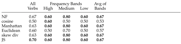
4.2.1 Experimental Results.On dataset1, our network flow distance performs better than or as well as all other measures on the individual frequency bands, as shown in Table 1. On all verbs combined (the “All” column) the performance of our method is not the best, although the Wilcoxon test shows no significant difference between the rankings of NF and the best measure (Manhattan). (The difference in rankings between NF and all other measures is significant.)

Table 1

Accuracies on dataset1 by the network flow method (NF), cosine, Manhattan distance, Euclidean distance, skew divergence (skew div), and Jensen-Shannon divergence (JS). Best accuracies in each condition are shown inboldface.

All Frequency Bands Avg of Verbs High Medium Low Bands

NF 0.60 0.70 0.70 0.70 0.70

cosine 0.57 0.60 0.60 0.60 0.60 Manhattan 0.63 0.70 0.70 0.70 0.70

Euclidean 0.47 0.40 0.50 0.40 0.43 skew div 0.57 0.60 0.60 0.50 0.57

JS 0.60 0.70 0.60 0.70 0.67

Table 2

Accuracies on dataset2 by the network flow method (NF), cosine, Manhattan distance, Euclidean distance, skew divergence (skew div), and Jensen-Shannon divergence (JS). Best accuracies in each condition are shown inboldface.

All Frequency Bands Avg of Verbs High Medium Low Bands

NF 0.67 0.60 0.80 0.60 0.67

cosine 0.50 0.60 0.50 0.50 0.53 Manhattan 0.63 0.60 0.80 0.60 0.67

Euclidean 0.60 0.50 0.70 0.50 0.57 skew div 0.63 0.60 0.80 0.60 0.67

JS 0.70 0.60 0.80 0.60 0.67

between the two slots and high frequency verbs tend to have larger distances. This is due to the fact that higher frequency verbs typically occur with a wider range of nouns, leading to a more dispersed semantic profile (i.e., a larger number of concepts). As a result, the best threshold for separating the alternating and non-alternating verbs differs across the frequency bands, and the threshold for all verbs together lies in between the thresholds for the high and low frequency bands. When classifying all verbs, the frequency effect may result in more false positives for low frequency verbs (which have generally smaller distance values), and more false negatives for high frequency verbs (which have generally larger distance values). The column labelled “Avg” in Table 1 shows the performance when averaging the results across the individual frequency bands. For most methods, including ours, the “Avg” results are much better than when considering all verbs together (the “All” column).

Table 2 reports the performance on dataset2, which is similar to that on dataset1. Again, we find that our method is tied for the best performance in every condition except for all verbs combined. (Here we find that all four methods over .60 accuracy in the “All” condition have statistically indistinguishable rankings of the experimental items.) On this data set, taking the average of the frequency bands does not help performance of our method compared to “All,” but neither does it hurt (and for most methods “Avg” does better or the same as “All”). We conclude that separating items by frequency may be required to achieve robust results in this type of task.

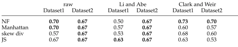
Table 3

Average accuracies by the network flow method (NF), Manhattan distance (Man), skew divergence (skew div), and Jensen-Shannon divergence (JS) on different profiles: original (“raw”), Li and Abe, and Clark and Weir profiles. Best accuracies in each condition are shown in

boldface.

raw Li and Abe Clark and Weir

Dataset1 Dataset2 Dataset1 Dataset2 Dataset1 Dataset2

NF 0.70 0.67 0.50 0.67 0.73 0.70

Manhattan 0.70 0.67 0.57 0.67 0.60 0.57

skew div 0.57 0.67 0.53 0.67 0.68 0.60

JS 0.67 0.67 0.63 0.67 0.63 0.53

relatively small amounts of data per verb (with profiles averaging about 900 nodes in size), it is possible that the raw profiles suffer from a sparse data problem and are not sufficiently capturing the conceptual similarities among alternating slots. McCarthy (2000) addressed this issue by using a technique for generalizing concept nodes prior to comparing profiles. We explore this issue next.

4.2.2 Comparing Different Profile Generation Methods.Our experiments use semantic pro-files created directly from the word frequencies, as described earlier. However, research has explored the possibility of generalizing this kind of “raw” data to a semantic profile that more appropriately reflects the coherent concepts expressed in the original set of weighted concept nodes. This can be especially useful when creating semantic profiles from small amounts of data, given the noise introduced in the mapping of words to concepts.6To explore the effect of different profile generation methods on this task, we consider here two approaches, that of Li and Abe (1998) and Clark and Weir (2002). Both these methods start with a semantic profile generated as described in Section 3 and attempt to find the set of nodes in the ontology that appropriately generalize the concepts in the “raw” profile.

Table 3 compares the performance of the network flow distance with that of several other measures on the original (“raw”) profiles, the Li and Abe profiles, and the Clark and Weir profiles. Results are reported for the average of the individual frequency bands, since that produced the best results overall in our earlier experiments. The results for cosine and Euclidean distance are omitted, because they perform worse overall than the other measures.7

The best results across both data sets are achieved by our network flow method on the Clark and Weir profiles. Considering the results across all profile types, the network flow approach is most consistent, achieving the best (or tied for best) performance in but one condition (dataset1 with Li and Abe profiles). The distributional methods

6 Because we divide the frequency of a word uniformly among all the word’s concepts, with no attempt at disambiguation or informed weighting, much noise is introduced. Given the small amounts of data, the noise may be sufficient to mislead our network flow method.

(Manhattan, skew div, JS) in almost all cases perform worse on the generalized profiles than on the “raw” profiles. (The one exception is that skew divergence does better on dataset1 on the Clark and Weir profiles.)

Overall, then, it seems that raw data is likely best for a purely distributional method, but the Clark and Weir profiles enable the network flow method to outperform them by exploiting the graph structure of the ontology. Indeed, when comparing our method to the others on the Clark and Weir profiles for the individual frequency bands (not shown in the table), we find that much of our performance advantage comes on the low frequency verbs. This indicates that the combination of our method with a suitable generalization technique is especially important when dealing with sparse data.

We examine the data further to discover why the Li and Abe profiles yield poorer performance in most cases on dataset1. We find that Li and Abe’s (1998) method tends to generate profiles with more general concepts. For example, when given an original set of concepts such asEdam,Brie,Sockeye, andChinook, the method may produce a single general concept such asfoodinstead of the two conceptscheeseandsalmonthat capture the two kinds of food that are indicated. The loss of semantic information from using overly general concepts may produce the decrease in performance.

For comparison, we also apply McCarthy’s (2000) method to our dataset2, and find that it achieves only 0.60 on all verbs and 0.53 averaged over the three frequency bands. Her method is especially poor on low frequency verbs (below chance at 0.40). We hypothesize that her method is less robust to low frequency counts because it may overgeneralize the data by first applying Li and Abe’s (1998) method, and then generalizing the nodes even further.

We see that although some amount of generalization of the semantic profiles is useful in this task, overgeneralization may be harmful. We leave it to future work to explore the interaction of our network flow method with different types of profile generation across various tasks. Because the next two tasks we consider use larger amounts of data, we only experiment with raw profiles in these cases.

5. Task 2: Name Disambiguation

Interest in the NLP problem of name disambiguation has increased as the growth of the World Wide Web has led to large numbers of ambiguous name references in on-line text. For example, Web sites or documents containing the nameJohn Edwardsmay refer to the U.S. presidential candidate for 2008, an NBA basketball player, or a British medical geneticist. An ambiguous name may be resolved by comparing its local textual context—the set of words it co-occurs with—with the local textual contexts of the name when its reference is known. For example, the text surrounding the nameJohn Edwards in its various uses are very likely to include distinguishing words such aspoliticianvs. gamevs.research. Many approaches have been proposed for resolving name ambiguity by using distributional methods over contextual information (Xu, Liu, and Gong 2003; Han, Zha, and Giles 2005; Pedersen, Purandare, and Kulkarni 2005).

and a diplomat (Tajik and Rolf Ekeus) form another. This task was established by Pedersen, Purandare, and Kulkarni (2005) to provide “annotated” experimental data (with each text indicating the correct name) without the need for expensive manual annotation.

In Pedersen, Purandare, and Kulkarni (2005), an unsupervised method of name discrimination through text clustering was used to address this task. This is infeasible for a method like ours, in which each distance calculation requires access to an ontology. (The worst-case complexity of clustering with our method is quadratic in the size of the ontology used; a detailed discussion can be found in Tsang and Stevenson [2006].) In-stead, we use a supervised methodology, but experiment with varying small amounts of data in a minimally supervised approach. Although our method requires extra manual effort in the form of data annotation for training, we find that the amount of annotated data required is modest.

5.1 Experimental Methodology

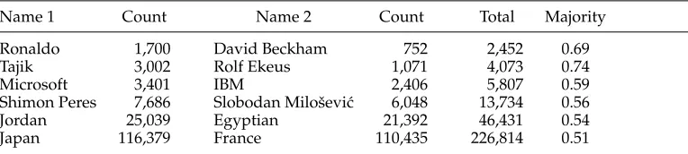
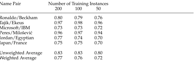
5.1.1 Corpus Data. We use Pedersen, Purandare, and Kulkarni’s (2005) data set, which was taken from the Agence France-Press English Service portion of the GigaWord English corpus distributed by the Linguistic Data Consortium. They extracted the local context of six pairs of names of varying confusability, including: the names of two soccer players (Ronaldo and David Beckham); an ethnic group and a diplomat (Tajik and Rolf Ekeus); two companies (Microsoft and IBM); two politicians (Shimon Peres and Slobodan Miloˇsevi´c); a nation and a nationality (Jordan and Egyptian); and two countries (France and Japan). For each name instance, the extracted text consists of 50 words (25 words to the left and to the right of the target name), with the target name obfuscated. For example, for the task of distinguishingDavid BeckhamandRonaldo, the target name in each instance becomesDavid BeckhamRonaldo. The original name in each instance is retained only for evaluating the results (and for training, in the case of our method, as described subsequently). (Note that this approach to data creation avoids the use of manually annotated data for this experimental task, but in an actual application, manual annotation of truly ambiguous names would be necessary.) Each pair of names thus serves as one of six name disambiguation tasks. Table 4 shows the number of instances per task (name pair). The “Majority” column also indicates the relative frequency of the majority name in each pair, which we adopt as the baseline accuracy.

5.1.2 Classification Using the NetworkFlow Method.As mentioned previously, we take a supervised approach, in which name instances are classified with the use of training

Table 4

The pairs to be identified, the raw frequencies, and the relative frequency of the majority name.

Name 1 Count Name 2 Count Total Majority

Ronaldo 1,700 David Beckham 752 2,452 0.69

Tajik 3,002 Rolf Ekeus 1,071 4,073 0.74

Microsoft 3,401 IBM 2,406 5,807 0.59

Shimon Peres 7,686 Slobodan Miloˇsevi´c 6,048 13,734 0.56

Jordan 25,039 Egyptian 21,392 46,431 0.54

data annotated by the original name in the instance. To generate our training data, we randomly select a portion of the instances for each of the 12 names. All the training instances for a name are used to form a single aggregate semantic profile, which serves as the gold-standard for that name. The remaining instances serve as test data; for each of these, we build an individual semantic profile. All profiles are generated as described in Section 3, namely, each frequency count for a word is distributed uniformly among the corresponding concepts in WordNet. A gold-standard profile is constructed in exactly the same way except that its word frequency vector is created by aggregating the word counts from all the relevant training instances. Note that there is nothing special about such a profile or how it is formed; it simply aggregates counts from multiple contexts.8

To classify a name instance, we measure the network-flow distance between the individual profile of the ambiguous instance and each of the two gold-standard profiles for that task. The name whose gold-standard profile has the shortest distance to the instance profile is the name assigned to the ambiguous instance. For example, assume we have a “David BeckhamRonaldo” instance to be classified. We compare its profile to each of the gold standard profiles for “David Beckham” and “Ronaldo” by measuring the distance between each of the two pairs of profiles. If the instance profile has a shorter distance to the profile for “David Beckham” than to that of “Ronaldo,” then it is classified as “David Beckham,” otherwise as “Ronaldo.”

5.1.3 Evaluation Methodology.We use the accuracy of labelling all instances as our eval-uation measure. To compare to prior results using F-measure, we report that in some tables. Because we label all instances, accuracy and F-measure are equivalent in our method, using 2rp/(r+p) as the definition of F-measure.

The random baseline for our task is the accuracy of labelling all instances with the predominant name, as shown in the “Majority” column of Table 4. Because we use the data set of Pedersen, Purandare, and Kulkarni (2005), we compare our performance to their distributional method (reporting their best results both with and without singular value decomposition). Because their method is an unsupervised one, we also train and test a supervised learner using distributional data (LIBSVM by Chang and Lin [2001]). For each set of training data, we remove stopwords and use the remaining words (with their frequencies) as input features for the SVM. We then obtain the optimal parameters (i.e., optimal values for cost and gamma in LIBSVM) by using 10-fold cross-validation over the training data. Finally, we perform classification on the test data using those parameters. This enables us to compare our results to a purely distributional method with access to the same training data.

Because our method is supervised, it is important to minimize the amount of annotated data required to build the gold-standard profiles. (Lengthy training time can also be an issue for a supervised method, but here “training” is the straightforward task of building an aggregate semantic profile.) Because it is unclear a priori what amount of training data is sufficient, we experiment with several quantities. We initially select 200 random instances per pair of names, respecting the relative proportions of the two names overall. (Two hundred instances constitute about 0.1–10% of the data per pair of names.) Subsequently, we decrease the quantity further, to half and one-quarter the original amount (100 and 50 instances, respectively) to observe how the

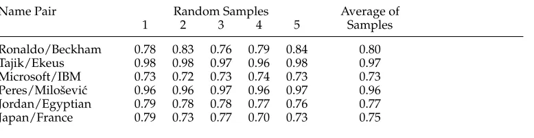
Table 5

Network flow results using 200 training instances on the random samples and their average performance.

Name Pair Random Samples Average of

1 2 3 4 5 Samples

Ronaldo/Beckham 0.78 0.83 0.76 0.79 0.84 0.80 Tajik/Ekeus 0.98 0.98 0.97 0.96 0.98 0.97 Microsoft/IBM 0.73 0.72 0.73 0.74 0.73 0.73 Peres/Miloˇsevi´c 0.96 0.96 0.97 0.96 0.97 0.96 Jordan/Egyptian 0.79 0.78 0.78 0.77 0.76 0.77 Japan/France 0.79 0.73 0.77 0.70 0.73 0.75

Table 6

Average results for the network flow (NF) results using 200 instances per gold-standard profile, SVM using 200 training vectors, and Ped05 and Ped05SVD(the best results without and with SVD, respectively). All results are F-measure (the same as accuracy for our method and SVM). The weighted average is calculated based on the number of instances in each pair of names. The best result for each name pair is indicated inboldface.

Name Pair Majority Ped05 Ped05SVD SVM200 NF200

Ronaldo/Beckham 0.69 0.73 0.65 0.85 0.80

Tajik/Ekeus 0.74 0.96 0.89 0.90 0.97

Microsoft/IBM 0.59 0.51 0.59 0.62 0.73

Peres/Miloˇsevi´c 0.56 0.97 0.94 0.90 0.96 Jordan/Egyptian 0.54 0.59 0.62 0.72 0.77

Japan/France 0.51 0.51 0.50 0.48 0.75

Unweighted Average 0.61 0.71 0.70 0.75 0.84

Weighted Average 0.53 0.55 0.55 0.55 0.77

performance is influenced by the amount of data used to construct the gold standard profiles.9To reduce the impact of possible skewed sampling of training data, we repeat the random sampling five times, with no overlap between the random samples. We report the performance of each sample set as well as the average over the five samples.

5.2 Results and Analysis

5.2.1 Initial Experiments.Table 5 shows the performance of our method over five random samples of 200 training instances per task. Observe that the performance over the five rounds varies very little (a maximum difference of 0.08, and most are much closer). This shows the robustness of our method to different make-ups of training data. Table 6 shows the average performance of our method, in comparison to the chance (majority) baseline, as well as the results produced by the unsupervised method of Pedersen, Purandare, and Kulkarni (2005) (with singular value decomposition [SVD] reported as

Ped05SVD, and without SVD as Ped05), and the supervised SVM on the same training

data as our method. Observe that our method not only significantly outperforms the random baseline, it is moreover the best performer among all the methods (paired t-test, p<0.05).

There are cases for which Pedersen, Purandare, and Kulkarni’s (2005) methods have at best chance performance (Microsoft/IBMandJapan/France). The authors suggest that these pairs of names arise in the context of news text in which there are “no consis-tently strong discriminating features” useful in the clustering algorithm. (Interestingly, this is the case even with SVD, where words are grouped into a small number of un-named concepts.) Even the SVM has difficulty with these pairs, also performing at just around chance. Yet our method performs well above chance for these pairs. In general, SVM produces results that are little better on average than the unsupervised results in Pedersen, Purandare, and Kulkarni (2005) (with some tasks performing better, and some worse). This shows that the performance improvement from the network flow method does not depend solely on access to training data. Instead, it seems that the use of ontological relations in calculating distance can significantly enhance the discriminatory power over simply using words.

Note that there is one difference between the data used in the SVM and the network flow experiments: The SVM is trained using all words as features, while only WordNet noun concepts are used in the network flow experiments. It is possible that using just nouns or a mapping of nouns to WordNet concepts could bring the performance of the SVM into line with our network flow measure. We thus perform two replications of the SVM experiments, one using only nouns as features and one using noun concepts as features (with the relevant frequencies as the feature values in both cases). However, both of these approaches produce little to no improvement over the all-words results reported in Table 6. We conclude that our network flow method is superior to, and more consistent than, the purely distributional methods, and that this difference is attributable to the integration of distributional and ontological (relational) information in our measure.

5.2.2 Reducing the Amount of Training Data.Because, in contrast to Pedersen, Purandare, and Kulkarni (2005), we use a supervised approach, we want to determine whether we can reduce our dependence on training data. Here, we report experiments using one-half (100 instances) and one-quarter (50 instances) of the training data used earlier. As before, we repeat the random sampling of the training instances five times in each case, and report the average performance here.

Table 7 shows the network flow performance for 200, 100, and 50 training instances. Numerically, the results do not differ by much when the training data is reduced from 200 to 100 instances, and a paired t-test finds the difference to be non-significant. The performance drop is more pronounced in the 50-instance experiment, where every pair of names shows some drop in performance compared to 100 instances. Here, a paired t-test shows that the performance drop in the 50-instance experiment is statistically significant (p=0.04). Despite this, we still outperform the other methods: Our results using 50 training instances are much better than those of Pedersen, Purandare, and Kulkarni (2005) in all but one task, and even better overall than the SVM in 200 training instances (compare the SVM column of Table 6).

Table 7

Average classification results of the network flow method using 200, 100, and 50 training data per classification task. The weighted average is calculated based on the number of test instances per task.

Name Pair Number of Training Instances

200 100 50

Ronaldo/Beckham 0.80 0.79 0.76

Tajik/Ekeus 0.97 0.98 0.96

Microsoft/IBM 0.73 0.73 0.72 Peres/Miloˇsevi´c 0.96 0.97 0.94 Jordan/Egyptian 0.77 0.74 0.70

Japan/France 0.75 0.75 0.70

Unweighted Average 0.83 0.83 0.80 Weighted Average 0.77 0.76 0.72

profiles to 20 and 5 instances per task, and observe a continual drop in performance. The performance of one task (Ronaldo/David Beckham) drops below chance with 20 training instances and another (Microsoft/IBM) drops below chance with 5. For this set of data, we conclude that 50 instances per task are required to provide enough discriminatory power for our method.

Although unsupervised methods have the advantage of requiring no training data, in our case, 50 to 100 training instances constitute only a very small portion of the data, as well as a small amount of annotation effort in absolute terms. We conclude that the (small) labelling effort is justified by the performance gain achieved using our minimally supervised approach.

6. Task 3: Document Classification

Document classification is an NLP task in which a previously unseen document is given a topic label (or a set of such labels) based on its subject matter. For example, a financial document discussing the fluctuation of crude oil prices may be labelled “commerce” or “crude oil” in the Reuters Corpus (Lewis et al. 2004). In our version of the task, each document has a single topic label. Document classification is typically performed by comparing the text of an unlabelled document to the text of documents whose topics (labels) are known, and assigning the label of the closest such document (Joachims 2002; Iwayama et al. 2003; Esuli, Fagni, and Sebastiani 2006; Nigam, McCallum, and Mitchell 2006). This task is thus similar to the name disambiguation task in the previous section, and our approach is similar as well: Here again, we form gold-standard profiles from a small collection of texts of known classes, and then compare each test instance to each of the gold-standard profiles. As in name disambiguation, we experiment with different amounts of training data for creating the gold-standard profiles.

6.1 Experimental Set-up

6.1.1 Corpus Data.Our data is a corpus of articles from 20 different Usenet newsgroups released by Mitchell (1999). Because each newsgroup corresponds to a topic, the articles can be classified using the (single) newsgroup label. We use the collection maintained by Rennie (2001), in which all the duplicates (cross-posts) are removed, resulting in 18,828 articles. The articles are approximately evenly distributed among the 20 newsgroups. Stopwords and article headers are removed before processing each text.

Work that relies on word frequency vectors to represent the texts in document classification has revealed the importance of preprocessing the word frequency data to emphasize those terms that are likely to be most meaningful. For example, word fre-quencies have typically been weighted by inverse document frefre-quencies (tf·idf) to lessen the impact of very common but less distinguishing words. According to Rennie (2001), their best system on the same corpus uses the log_logtf_idf+1 weighting scheme. In order to compare our system to theirs, we use this same word weighting scheme in the creation of the word vectors that are used to produce our semantic profiles. (We have experimented with using raw word frequencies as well as tf ·idf to pro-duce profiles. Both methods yield approximately the same results as the log_logtf_idf+1 frequency weighting scheme.)

6.1.2 Training and Evaluation.As mentioned before, we treat the classification task simi-larly to name disambiguation, taking a minimally supervised approach. We randomly select a small number of documents as training data for creating the gold-standard semantic profiles. We use 10 or 30 documents per newsgroup, or approximately 1–3% of the documents. The remaining documents are used as testing data. Again, we use a random sample of documents for each gold-standard profile, repeated five times to minimize the impact of a possible skewed sampling. We report the average accuracy over the five samples.

Because there are 20 possible topic labels, the random baseline is very low, at 5%. (Using the predominant label raises this only slightly.) A more informative evaluation of our method is to compare to a state-of-the-art approach that is purely distributional. A comparison to Rennie (2001) is natural, since we use the same data set. However, they trained an SVM on 30 documents per class and tested on 10% of the documents, repeated 10 times. Because our training approach differs somewhat (training on 10 or 30 documents per class, testing on all remaining documents, repeated 5 times), we also replicate their SVM experiment using our training and test sets. As in the name disambiguation task, we use the LIBSVM software package (Chang and Lin 2001) and tune the classifier in the training phase for the best SVM parameters prior to the testing. Also as in our name disambiguation task, we additionally train and test the SVM on just the nouns in a document (rather than all words), and also on the nouns mapped to concepts (with the relevant frequencies as the feature values in both cases). Thus we report results of the SVM on three different types of input frequency vectors: all words, nouns, and concepts.

6.2 Results and Analysis

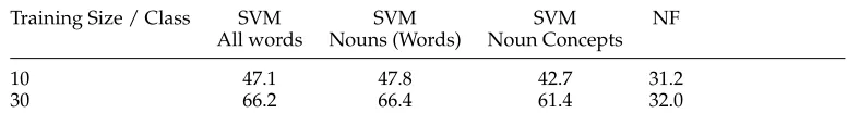
Table 8

Average classification results using 10 and 30 training documents per newsgroup.

Training Size / Class SVM SVM SVM NF

All words Nouns (Words) Noun Concepts

10 47.1 47.8 42.7 31.2

30 66.2 66.4 61.4 32.0

by Rennie (2001) using an SVM. One possible reason is that the SVM is trained on all words (minus stopwords and article headers), whereas our network flow method applies to noun concepts only. The SVM performance on noun-only data is similar to that of all words. Although there is a marked decrease in performance on the concept frequency vectors, SVM still outperforms our method.

The poorer SVM performance on concept frequencies suggests that concept fre-quency vectors are less easily distinguishable than word frefre-quency vectors. Recall, however, that we found no difference with these various training approaches for SVM in name disambiguation. It is possible that the mapping from words to concepts is a problem here because the full text is used, rather than a relatively small window around a target word. Because each word can map to multiple (potentially unrelated) concepts, the use of a larger, unconstrained bag of words may lead to a high degree of ambiguity, introducing more noise in the semantic profile than our method can handle. This may also explain why the network flow method does not improve with additional training data, showing virtually no improvement between 10 and 30 training instances (0.8% difference). We speculate that the amount of noise in a semantic profile based on the larger amount of text may increase along with the increase in the training size, offsetting any potential gain from having additional data.

If this hypothesis is correct, it is natural to ask why the SVM result using concepts shows a substantial increase in accuracy from 10 to 30 training documents. If larger texts yield nosier semantic profiles, why does this not negatively affect the SVM as well? This highlights a fundamental distinction of our approach: our method is novel because it finds the distance between conceptsas embedded in a graph (the ontology), not just between conceptvectors. Generally, our thesis is that this is an advantage of our model: It entails that all concepts generated from a text play a role in determining the distance of that text from another. As we noted earlier, this allows us to find similarity between texts that use related but not equivalent concepts. However, the performance of our method in this document classification task reveals a potential drawback of this property of our method. Because it takes all concepts into account in determining distance, it is more susceptible to noise. Figure 5 illustrates the problem. We see that the square and triangle profiles are noisy—that is, they each have a number of nodes that are not part of their coherent semantic content. These noisy aspects of the two profiles are less separated in ontological space, making the two profiles more similar according to our measure than their “true” semantic content would indicate. Because a vector representation of concepts does not form connections between differing concepts, it is not led astray in the way our method is.

Figure 5

Two noisy profiles, one represented by squares, the other by triangles.

exacerbated by the fact that, in using the full document, we may have a higher number of less relevant words than when a profile is formed from a more constrained set of words (as in verb alternation detection and name disambiguation). If this hypothesis is true, then the noisy (irrelevant) concepts should be distributed within each profile according to some prior probability distribution. If we knew that distribution, then we could “subtract out” the noise and form more semantically coherent profiles. Referring to Figure 5, the idea is that we would like to remove the small, dispersed squares and triangles, leaving only the larger ones that form a semantically more coherent set.

We test this idea, experimenting with two possible noise distributions. The first is simply the uniform distribution, and the second is a distribution determined empiri-cally using frequency counts from a domain-general corpus. For the latter, we determine a distribution over concepts based on the nouns in the BNC. Because the BNC is a balanced corpus, the distribution of its nouns can be considered a prior that is treatable as noise compared to the distribution in a newsgroup posting that is specific to a particular topic. In each case, we create a semantic profile representing the expected noise, and then “subtract” the resulting noise profile from each of our gold-standard semantic profiles in the document classification task. The “subtraction” is actually a process of setting to zero all of the semantic profile frequencies that are less than the noise value for that concept. Any node with a value higher than the noise value for that node is expected to be a potentially relevant concept. We leave such nodes at their original value so that they are more distinguished from the remaining values (now set to zero). Figure 6 illustrates the result of applying this kind of noise reduction to the profiles in Figure 5. We can see that low-frequency concept nodes are zeroed out, with higher frequency nodes maintaining their concept weight.

Table 9 presents the network flow results on the noise-subtracted data, showing a 3–5% increase in the performance using 30 training documents per class. The perfor-mance decreases with noise-subtraction when we have only 10 training documents per class, suggesting that there may not be enough data in this case to use this simplistic subtractive method.

Figure 6

The same two profiles in Figure 5. The profile masses that are “subtracted” are shaded in gray.

which may make it more similar to a balanced corpus than we have originally antic-ipated, thus what we are treating as a “noise” distribution in this case may not actually represent noise. That said, there is a small but notable increase even using the BNC noise distribution when we have sufficient training data. The idea of subtracting out noise seems promising, but we leave the appropriate representation of noise, and the mechanism for removing it effectively, as an area of future research.

7. Profile Density: A Measure of Coherence of Semantic Profiles

We have seen a performance difference across the three tasks we used in evaluation: the network flow method outperforms purely distributional measures on verb alterna-tion detecalterna-tion and name disambiguaalterna-tion, but does poorly on document classificaalterna-tion compared to a distributional approach. (See Table 10 for a summary of the results.) We use the same ontology (WordNet) and the same concept distance (number of edges) in our network flow measure across all three tasks, hence there must be some difference in the three data sets themselves that impacts the ability of our method to distinguish the semantic profiles corresponding to one class of data (one usage of an ambiguous name, for example) from the profiles of a different class of data (the other usage of the name). In this section, we develop a measure that can capture this property and explain the performance differential we have observed for our method.

Table 9

Average classification results using 30 and 10 training documents per newsgroup, using the original profiles (NF), and using profiles after the “noise subtraction” process described in the text (“NF−Uniform” and “NF−BNC” are results subtracting the uniform distribution and the BNC noun frequency distribution, respectively).

Training Size / Class NF NF−Uniform NF−BNC

10 31.2 28.2 27.4

Table 10

Summary of task-based results. The numbers in parentheses indicate the number of training instances used. The best result for each task is shown inbold.

Verb Alternation Detection random Manhattan skew div JS NF

Dataset1 Avg 0.50 0.70 0.57 0.67 0.70

Dataset2 Avg 0.50 0.67 0.67 0.67 0.67

Name Disambiguation random SVM (100) SVM (200) NF (100) NF (200)

Unweighted Avg 0.61 0.72 0.75 0.83 0.83

Weighted Avg 0.53 0.52 0.55 0.76 0.77

Document Classification random SVM (10) SVM (30) NF (10) NF (30)

20 newsgroups 0.05 0.43 0.61 0.31 0.32

7.1 Profile Coherence

Our goal is to find a property of individual semantic profiles that, when averaged across the profiles in a data set, indicates whether our method will be able to distinguish profiles of different classes in that data set. That is, we aim to learn about the overall separability of the classes in a data set by investigating the properties of individual profiles that constitute the data set. Our hypothesis is that the important factor for our method is what we refer to asprofile coherence: the degree to which profile mass is concentrated within a constrained space (or set of constrained spaces) of the ontology. The more spatially coherent the sets of weighted concepts are for the profiles in a data set, the more likely it is that our method will be able to distinguish contrasting profiles. Conversely, less coherent profiles, whose frequency mass is more distributed across a wider area of the ontology, will be more difficult to separate into classes. (Note that profile coherence is not a sufficient condition for data separability, but we hypothesize that it can be a useful indicator.)