Marco Kuhlmann
* Uppsala UniversitySyntactic representations based on word-to-word dependencies have a long-standing tradition in descriptive linguistics, and receive considerable interest in many applications. Nevertheless, dependency syntax has remained something of an island from a formal point of view. Moreover, most formalisms available for dependency grammar are restricted to projective analyses, and thus not able to support natural accounts of phenomena such as wh-movement and cross–serial dependencies. In this article we present a formalism for non-projective dependency grammar in the framework of linear context-free rewriting systems. A characteristic property of our formalism is a close correspondence between the non-projectivity of the dependency trees admitted by a grammar on the one hand, and the parsing complexity of the grammar on the other. We show that parsing with unrestricted grammars is intractable. We therefore study two constraints on non-projectivity, block-degree and well-nestedness. Jointly, these two constraints define a class of “mildly” non-projective dependency grammars that can be parsed in polynomial time. An evaluation on five dependency treebanks shows that these grammars have a good coverage of empirical data.
1. Introduction
Syntactic representations based on word-to-word dependencies have a long-standing tradition in descriptive linguistics. Since the seminal work of Tesni`ere (1959), they have become the basis for several linguistic theories, such as Functional Generative Description (Sgall, Hajiˇcov´a, and Panevov´a 1986), Meaning–Text Theory (Mel’ˇcuk 1988), and Word Grammar (Hudson 2007). In recent years they have also been used for a wide range of practical applications, such as information extraction, machine translation, and question answering. We ascribe the widespread interest in dependency structures to their intuitive appeal, their conceptual simplicity, and in particular to the availability of accurate and efficient dependency parsers for a wide range of languages (Buchholz and Marsi 2006; Nivre et al. 2007).
Although there exist both a considerable practical interest and an extensive lin-guistic literature, dependency syntax has remained something of an island from a formal point of view. In particular, there are relatively few results that bridge between dependency syntax and other traditions, such as phrase structure or categorial syntax.
∗ Department of Linguistics and Philology, Box 635, 751 26 Uppsala, Sweden. E-mail:[email protected].
Submission received: 17 December 2009; revised submission received: 3 April 2012; accepted for publication: 24 May 2012.
Figure 1
Nested dependencies and cross–serial dependencies.
This makes it hard to gauge the similarities and differences between the paradigms, and hampers the exchange of linguistic resources and computational methods. An overarching goal of this article is to bring dependency grammar closer to the mainland of formal study.
One of the few bridging results for dependency grammar is thanks to Gaifman (1965), who studied a formalism that we will refer to as Hays–Gaifman grammar, and proved it to be weakly equivalent to context-free phrase structure grammar. Although this result is of fundamental importance from a theoretical point of view, its practical usefulness is limited. In particular, Hays–Gaifman grammar is restricted to projective dependency structures, which is similar to the familiar restriction to contiguous con-stituents. Yet, non-projective dependencies naturally arise in the analysis of natural language. One classic example of this is the phenomenon of cross–serial dependencies in Dutch. In this language, the nominal arguments of verbs that also select an infinitival complement occur in the same order as the verbs themselves:
(i) dat Jan1 Piet2 Marie3 zag1 helpen2 lezen3 (Dutch) that Jan Piet Marie saw help read
‘that Jan saw Piet help Marie read’
In German, the order of the nominal arguments instead inverts the verb order:
(ii) dass Jan1 Piet2 Marie3 lesen3 helfen2 sah1 (German) that Jan Piet Marie read help saw
Figure 1 shows dependency trees for the two examples.1 The German linearization gives rise to a projective structure, where the verb–argument dependencies are nested within each other, whereas the Dutch linearization induces a non-projective structure with crossing edges. To account for such structures we need to turn to formalisms more expressive than Hays–Gaifman grammars.
In this article we present a formalism for non-projective dependency grammar based on linear context-free rewriting systems (LCFRSs) (Vijay-Shanker, Weir, and Joshi 1987; Weir 1988). This framework was introduced to facilitate the comparison of various
grammar formalisms, including standard context-free grammar, tree-adjoining gram-mar (Joshi and Schabes 1997), and combinatory categorial gramgram-mar (Steedman and Baldridge 2011). It also comprises, among others, multiple context-free grammars (Seki et al. 1991), minimalist grammars (Michaelis 1998), and simple range concatenation grammars (Boullier 2004).
The article is structured as follows. In Section 2 we provide the technical back-ground to our work; in particular, we introduce our terminology and notation for linear context-free rewriting systems. An LCFRS generates a set of terms (formal expressions) which are interpreted as derivation trees of objects from some domain. Each term also has a secondary interpretation under which it denotes a tuple of strings, representing the string yield of the derived object. In Section 3 we introduce the central notion of a lexicalized linear context-free rewriting system, which is an LCFRS in which each rule of the grammar is associated with an overt lexical item, representing a syntactic head (cf. Schabes, Abeill´e, and Joshi 1988 and Schabes 1990). We show that this property gives rise to an additional interpretation under which each term denotes a dependency tree on its yield. With this interpretation, lexicalized LCFRSs can be used as dependency grammars.
In Section 4 we show how to acquire lexicalized LCFRSs from dependency tree-banks. This works in much the same way as the extraction of context-free grammars from phrase structure treebanks (cf. Charniak 1996), except that the derivation trees of dependency trees are not immediately accessible in the treebank. We therefore present an efficient algorithm for computing a canonical derivation tree for an input depen-dency tree; from this derivation tree, the rules of the grammar can be extracted in a straightforward way. The algorithm was originally published by Kuhlmann and Satta (2009). It produces a restricted type of lexicalized LCFRS that we call “canonical.” In Section 5 we provide a declarative characterization of this class of grammars, and show that every lexicalized LCFRS is (strongly) equivalent to a canonical one, in the sense that it induces the same set of dependency trees.
In Section 6 we present a simple parsing algorithm for LCFRSs. Although the runtime of this algorithm is polynomial in the length of the sentence, the degree of the polynomial depends on two grammar-specific measures called fan-out and rank. We show that even in the restricted case of canonical grammars, parsing is an NP-hard problem. It is important therefore to keep the fan-out and the rank of a grammar as low as possible, and much of the recent work on LCFRSs has been devoted to the development of techniques that optimize parsing complexity in various scenarios G ´omez-Rodr´ıguez and Satta 2009; G ´omez-Rodr´ıguez et al. 2009; Kuhlmann and Satta 2009; Gildea 2010; G ´omez-Rodr´ıguez, Kuhlmann, and Satta 2010; Sagot and Satta 2010; and Crescenzi et al. 2011).
In this article we explore the impact of non-projectivity on parsing complexity. In Section 7 we present the structural correspondent of the fan-out of a lexicalized LCFRS, a measure calledblock-degree(or gap-degree) (Holan et al. 1998). Although there is no theoretical upper bound on the block-degree of the dependency trees needed for linguistic analysis, we provide evidence from several dependency treebanks showing that, from a practical point of view, this upper bound can be put at a value of as low as 2. In Section 8 we study a second constraint on non-projectivity calledwell-nestedness
(Bodirsky, Kuhlmann, and M ¨ohl 2005), and show that its presence facilitates tractable parsing. This comes at the cost of a small loss in coverage on treebank data. Bounded block-degree and well-nestedness jointly define a class of “mildly” non-projective dependency grammars that can be parsed in polynomial time.
2. Technical Background
We assume basic familiarity with linear context-free rewriting systems (see, e.g., Vijay-Shanker, Weir, and Joshi 1987 and Weir 1988) and only review the terminology and notation that we use in this article.
A linear context-free rewriting system (LCFRS) is a structure G=(N,Σ,P,S) where N is a set of nonterminals, Σ is a set of function symbols, P is a finite set of production rules, andS∈Nis a distinguished start symbol. Rules take the form
A0 →f(A1,. . .,Am) (1)
wheref is a function symbol and theAiare nonterminals. Rules are used for rewriting in the same way as in a context-free grammar, with the function symbols acting as terminals. The outcome of the rewriting process is a set T(G) of terms, tree-formed expressions built from function symbols. Each term is then associated with a string yield, more specifically atupleof strings. For this, every function symbolf comes with ayield functionthat specifies how to compute the yield of a termf(t1,. . .,tm) from the yields of its subtermsti. Yield functions are defined by equations
f(x1,1,. . .,x1,k1,. . .,xm,1,. . .,xm,km) = α1,. . .,αk0 (2)
where the tuple on the right-hand side consists of strings over the variables on the left-hand side and some given alphabet of yield symbols, and contains exactly one occurrence of each variable. For a yield functionf defined by an equation of this form, we say thatf is oftypek1· · ·km→k0, denoted byf :k1· · ·km→k0. To guarantee that the string yield of a term is well-defined, each nonterminal A is associated with a
fan-outϕ(A)≥1, and it is required that for every rule (1),
f :ϕ(A1)· · ·ϕ(Am)→ϕ(A0)
In Equation (2), the valuesmandk0are called therankand thefan-outoff, respectively. The rank and the fan-out of an LCFRS are the maximal rank and fan-out of its yield functions.
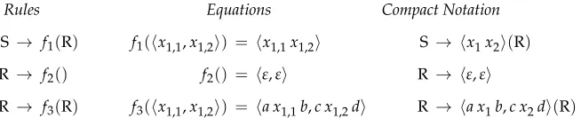
Example 1
Figure 2 shows an example of an LCFRS for the language{ anbncndn |n≥0}.
[image:4.486.51.378.566.637.2]Equation (2) is uniquely determined by the tuple on the right-hand side of the equation. We call this tuple the template of the yield function f, and use it as the canonical function symbol for f. This gives rise to a compact notation for LCFRSs,
Figure 2
illustrated in the right column of Figure 2. In this notation, to save some subscripts, we use the following shorthands for variables:x andx1 forx1,1;x2 forx1,2;x3 forx1,3; yandy1forx2,1;y2forx2,2;y3forx2,3.
3. Lexicalized LCFRSs as Dependency Grammars
Recall the following examples for verb–argument dependencies in German and Dutch from Section 1:
(iii) dass Jan1 Piet2 Marie3 lesen3 helfen2 sah1 (German) that Jan Piet Marie read help saw
(iv) dat Jan1 Piet2 Marie3 zag1 helpen2 lezen3 (Dutch) that Jan Piet Marie saw help read
‘that Jan saw Piet help Marie read’
Figure 3 shows the production rules of two linear context-free rewriting systems (one for German, one for Dutch) that generate these examples. The grammars arelexicalizedin the sense that each of their yield functions is associated with a lexical item, such assahor zag(cf. Schabes, Abeill´e, and Joshi 1988 and Schabes 1990). Productions with lexicalized yield functions can be read as dependency rules. For example, the rules
V→ x y sah(N, V) (German) V→ x y1zag y2(N, V) (Dutch)
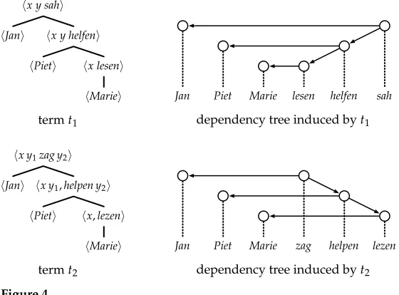
can be read as stating that the verbto seerequires two dependents, one noun (N) and one verb (V). Based on this reading, every term generated by a lexicalized LCFRS does not only yield a tuple of strings, but also induces a dependency tree on these strings: Each parent–child relation in the term represents a dependency between the associated lexical items (cf. Rambow and Joshi 1997). Thus every lexicalized LCFRS can be reinterpreted as a dependency grammar. To illustrate the idea, Figure 4 shows (the tree representations of) two terms generated by the grammarsG1andG2, together with the dependency trees induced by them. Note that these are the same trees that we gave for (iii) and (iv) in Figure 1.
Our goal for the remainder of this section is to make the notion of induction formally precise. To this end we will reinterpret the yield functions of lexicalized LCFRSs as operations on dependency trees.
Figure 3
Figure 4
Lexicalized linear context-free rewriting systems induce dependency trees.
3.1 Dependency Trees
By a dependency tree, we mean a pair (w, D), wherew is a tuple of strings, andDis a tree-shaped graph whose nodes correspond to the occurrences of symbols inw, and whose edges represent dependency relations between these occurrences. We identify occurrences inw by pairs (i,j) of integers, where i indexes the component of w that contains the occurrence, and j specifies the linear position of the occurrence within that component. We can then formally define a dependency graph for a tuple of strings
w = a1,1· · ·a1,n1,. . .,ak,1· · ·ak,nk
as a directed graphG=(V,E) where
V = {(i,j)|1≤i≤k, 1≤j≤ni} and E ⊆ V×V
We useuandvas variables for nodes, and denote edges (u,v) asu→v. Adependency tree D for w is a dependency graph for w in which there exists a root node r such that for any node u, there is exactly one directed path from r to u. A dependency tree is called simple if w consists of a single stringw. In this case, we write the de-pendency tree as (w,D), and identify occurrences by their linear positionsjinw, with 1≤j≤ |w|.
Example 2
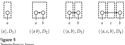
Figure 5
Dependency trees.
component; however, we usually omit the box when there is only one component. WritingDiasDi=(Vi,Ei) we have:
V1 = {(1, 1)} E1 = {}
V2 = {(1, 1), (1, 2)} E2 = {(1, 1)→(1, 2)}
V3 = {(1, 1), (2, 1)} E3 = {(1, 1)→(2, 1)}
V4 = {(1, 1), (3, 1)} E4 = {(1, 1)→(3, 1)}
We use standard terminology from graph theory for dependency trees and the relations between their nodes. In particular, for a nodeu, the set ofdescendantsofu, which we denote byu, is the set of nodes that can be reached fromuby following a directed path consisting of zero or more edges. We writeu<vto express that the nodeu precedes the nodevwhen reading the yield from left to right. Formally, precedence is the lexicographical order on occurrences:
(i1,j1)<(i2,j2) if and only if eitheri1<i2or (i1=i2andj1<j2)
3.2 Operations on Dependency Trees
A yield functionf is calledlexicalizedif its template contains exactly one yield symbol, representing a lexical item; this symbol is then called the anchor of f. With every lexicalized yield functionfwe associate an operationfon dependency trees as follows. Letw1,. . .,wm,wbe tuples of strings such that
f(w1,. . .,wm) = w
and let Di be a dependency tree for wi. By the definition of yield functions, every occurrenceuin an input tuplewicorresponds to exactly one occurrence in the output tuple w; we denote this occurrence by ¯ u. LetG be the dependency graph for w that has an edge ¯u→v¯ whenever there is an edgeu→vin someDi, and no other edges. Becausef is lexicalized, there is exactly one occurrencerin the output tuplewthat does not correspond to any occurrence in somewi; this is the occurrence of the anchor off. LetDbe the dependency tree forwthat is obtained by adding to the graphGall edges of the formr→r¯i, whereriis the root node ofDi. By this construction, the occurrencer of the anchor becomes the root node ofD, and the root nodes of the input dependency treesDibecome its dependents. We then define
Figure 6
Operations on dependency trees.
Example 3
We consider a concrete application of an operation on dependency trees, illustrated in Figure 6. In this example we have
f =x1b,y x2 w1=a,e w2=c d w =f(w1,w2)=a b,c d e
and the dependency treesD1,D2are defined as
D1 = ({(1, 1), (2, 1)},{(1, 1)→(2, 1)}) D2 = ({(1, 1), (1, 2)},{(1, 1)→(1, 2)})
We show thatf((w1,D1), (w2,D2))=(w, D), whereD=(V,E) with
V = {(1, 1), (1, 2), (2, 1), (2, 2), (2, 3)}
E = {(1, 1)→(2, 3), (1, 2)→(1, 1), (1, 2)→(2, 1), (2, 1)→(2, 2)}
The correspondences between the occurrences u in the input tuples and the occur-rences ¯uin the output tuple are as follows:
forw1: (1, 1)=(1, 1) , (2, 1)=(2, 3) forw2: (1, 1)=(2, 1) , (1, 2)=(2, 2)
By copying the edges from the input dependency trees, we obtain the intermediate dependency graphG=(V,E) forw, where
E = {(1, 1)→(2, 3), (2, 1)→(2, 2)}
The occurrencerof the anchorboff inw is (1, 2); the nodes ofGthat correspond to the root nodes ofD1 andD2 are ¯r1=(1, 1) and ¯r2=(2, 1). The dependency tree Dis obtained by adding the edgesr→r¯1andr→r¯2toG.
4. Extraction of Dependency Grammars
We now show how to extract lexicalized linear context-free rewriting systems from dependency treebanks. To this end, we adapt the standard technique for extracting context-free grammars from phrase structure treebanks (Charniak 1996).
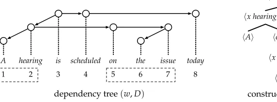
Figure 7
A dependency tree and one of its construction trees.
To extract a lexicalized LCFRS from a dependency treebank we proceed as follows. First, for each dependency tree (w,D) in the treebank, we compute aconstruction tree, a termtover yield functions that induces (w,D). Then we collect a set of production rules, one rule for each node of the construction trees. As an example, consider Fig-ure 7, which shows a dependency tree with one of its construction trees. (The analysis is taken from K ¨ubler, McDonald, and Nivre [2009].) From this construction tree we extract the following rules. The nonterminals (in bold) represent linear positions of nodes.
1→ A 5→ on x(7)
2→ x hearing,y(1,5) 6→ the
3→ x1is y1x2y2(2,4) 7→ x issue(6) 4→ scheduled,x(8) 8→ today
Rules like these can serve as the starting point for practical systems for data-driven, non-projective dependency parsing (Maier and Kallmeyer 2010).
Because the extraction of rules from construction trees is straightforward, the prob-lem that we focus on in this section is how to obtain these trees in the first place. Our procedure for computing construction trees is based on the concept of “blocks.”
4.1 Blocks
Let D be a dependency tree. A segment of D is a contiguous, non-empty sequence of nodes of D, all of which belong to the same component of the string yield. Thus a segment contains its endpoints, as well as all nodes between the endpoints in the precedence order. For a nodeu ofD, ablockof u is a longest segment consisting of descendants ofu. This means that the left endpoint of a block ofueither is the first node in its component, or is preceded by a node that is not a descendant ofu. A symmetric property holds for the right endpoint.
Example 4
We useuandvas variables for blocks. Extending the precedence order on nodes, we say that a blockuprecedes a blockv, denoted byu<v, if the right endpoint ofu precedes the left endpoint ofv.
4.2 Computing Canonical Construction Trees
To obtain a canonical construction tree t for a dependency tree (w,D) we label each nodeuofDwith a yield functionfas follows. Letwbe the tuple consisting of the blocks ofu, in the order of their precedence, and letw1,. . .,wmbe the corresponding tuples for the children ofu. We may view blocks as strings of nodes. Taking this view, we compute the (unique) yield functiongwith the property that
g(w1,. . .,wm) = w
The anchor of g is the node u, the rank of g corresponds to the number of children of u, the variables in the template ofgrepresent the blocks of these children, and the components of the template represent the blocks ofu. To obtainf, we take the template ofgand replace the occurrence ofuwith the corresponding lexical item.
Example 5
Node 2 of the dependency tree shown in Figure 7 has two children, 1 and 5. We have
w = 1 2, 5 6 7 w1 = 1 w2 = 5 6 7 g = x2,y f = x hearing,y
Note that in order to properly define f we need to assume some order on the children of u. The function g (and hence the construction tree t) is unique up to the specific choice of this order. In the following we assume that children are ordered from left to right based on the position of their leftmost descendants.
4.3 Computing the Blocks of a Dependency Tree
The algorithmically most interesting part of our extraction procedure is the computation of the yield function g. The template of g is uniquely determined by the left-to-right sequence of the endpoints of the blocks ofuand its children. An efficient algorithm that can be used to compute these sequences is given in Table 1.
Table 1
Computing the blocks of a simple dependency tree.
Input:a stringwand a simple dependency treeDforw
1: current← ⊥; markcurrent
2: for eachnodenextofDfrom 1 to|w|do
3: lca←next; stack←[]
4: whilelcais not markeddo loop 1
5: pushlcatostack; lca←the parent oflca
6: whilecurrent=lcado loop 2
7: next−1 is the right endpoint of a block ofcurrent
8: move up fromcurrentto the parent ofcurrent
9: unmarkcurrent; current←the parent ofcurrent
10: whilestackis not emptydo loop 3
11: current←popstack; markcurrent
12: move down from the parent ofcurrenttocurrent
13: nextis the left endpoint of a block ofcurrent
14: arrive atnext; at this point,current=next
15: whilecurrent=⊥do loop 4
16: |w|is the right endpoint of a block ofcurrent
17: move up fromcurrentto the parent ofcurrent
18: unmarkcurrent; current←the parent ofcurrent
4.3.2 Runtime Analysis. We analyze the runtime of our algorithm. Let m be the total number of blocks ofD. Let us writenifor the total number of iterations of theithwhile loop, and letn=n1+n2+n3+n4. Under the reasonable assumption that every line in Table 1 can be executed in constant time, the runtime of the algorithm clearly is inO(n). Because each iteration of loop 2 and loop 4 determines the right endpoint of a block, we haven2+n4 =m. Similarly, as each iteration of loop 3 fixes the left endpoint of a block, we haven3 =m. To determinen1, we note that every node that is pushed to the auxiliary stack in loop 1 is popped again in loop 3; therefore,n1=n3 =m. Putting everything together, we haven=3m, and we conclude that the runtime of the algorithm is inO(m). Note that this runtime is asymptotically optimal for the task we are considering.
5. Canonical Grammars
Our extraction technique produces a restricted type of lexicalized linear context-free rewriting system that we will refer to as “canonical.” In this section we provide a declarative characterization of these grammars, and show that every lexicalized LCFRS is equivalent to a canonical one.
5.1 Definition of Canonical Grammars
We are interested in a syntactic characterization of the yield functions that can occur in extracted grammars. We give such a characterization in terms of four properties, stated in the following. We use the following terminology and notation. Consider a yield function
f :k1· · ·km →k, f =α1,. . .,αk
components in the template off represent the blocks of a nodeu, and the variables in the template represent the blocks of the children of u. For a variablexi,j we calli the argument indexandjthecomponent indexof the variable.
Property 1
For all 1≤i1,i2≤m, ifi1<i2thenxi1,1<f xi2,1.
This property is an artifact of our decision to order the children of a node from left to right based on the position of their leftmost descendants. A variable with argument index i represents a block of theith child ofu in that order. An example of a yield function that does not have Property 1 isx2,1x1,1, which defines a kind of “reverse concatenation operation.”
Property 2
For all 1≤i≤mand 1≤j1,j2 ≤ki, ifj1<j2thenxi,j1 <f xi,j2.
This property reflects that, in our extraction procedure, the variablexi,j represents the jth block of theith child ofu, where the blocks of a node are ordered from left to right based on their precedence. An example of a yield function that violates the property isx1,2x1,1, which defines a kind ofswapping operation. In the literature on LCFRSs and related formalisms, yield functions with Property 2 have been called monotone
(Michaelis 2001; Kracht 2003), ordered (Villemonte de la Clergerie 2002; Kallmeyer 2010), andnon-permuting(Kanazawa 2009).
Property 3
No componentαhis the empty string.
This property, which is similar to ε-freeness as known from context-free grammars, has been discussed for multiple context-free grammars (Seki et al. 1991, Property N3 in Lemma 2.2) and range concatenation grammars (Boullier 1998, Section 5.1). For our extracted grammars it holds because each componentαhrepresents a block, and blocks are always non-empty.
Property 4
No componentαhcontains a substring of the formxi,j1xi,j2.
This property, which does not seem to have been discussed in the literature before, is a reflection of the facts that variables with the same argument index represent blocks of the same child node, and that these blocks arelongestsegments of descendants.
A yield function with Properties 1–4 is calledcanonical. An LCFRS is canonical if all of its yield functions are canonical.
Lemma 1
A lexicalized LCFRS is canonical if and only if it can be extracted from a dependency treebank using the technique presented in Section 4.
Proof
a dependency tree such that the construction tree extracted for this dependency tree containsf. This is an easy exercise.
We conclude by noting that Properties 2–4 are also shared by the treebank grammars extracted from constituency treebanks using the technique by Maier and Søgaard (2008).
5.2 Equivalence Between General and Canonical Grammars
Two lexicalized LCFRSs are calledstrongly equivalentif they induce the same set of dependency trees. We show the following equivalence result:
Lemma 2
For every lexicalized LCFRS G one can construct a strongly equivalent lexicalized LCFRSGsuch thatGis canonical.
Proof
Our proof of this lemma uses two normal-form results about multiple context-free grammars: Michaelis (2001, Section 2.4) provides a construction that transforms a mul-tiple context-free grammar into a weakly equivalent mulmul-tiple context-free grammar in which all rules satisfy Property 2, and Seki et al. (1991, Lemma 2.2) present a corre-sponding construction for Property 3. Whereas both constructions are only quoted to preserve weak equivalence, we can verify that, in the special case where the input grammar is a lexicalized LCFRS, they also preserve the set of induced dependency trees. To complete the proof of Lemma 2, we show that every lexicalized LCFRS can be cast into normal forms that satisfy Property 1 and Property 4. It is not hard then to combine the four constructions into a single one that simultaneously establishes all properties of canonical yield functions.
Lemma 3
For every lexicalized LCFRS G one can construct a strongly equivalent lexicalized LCFRSGsuch thatGonly contains yield functions which satisfy Property 1.
Proof
The proof is very simple. Intuitively, Property 1 enforces a canonical naming of the arguments of yield functions. To establish it, we determine, for every yield functionf, a permutation πthat renames the argument indices of the variables occurring in the template offin such a way that the template meets Property 1. This renaming gives rise to a modified yield functionfπ. We then replace every ruleA→f(A1,. . .,Am) with the modified ruleA→fπ(Aπ(1),. . .,Aπ(m)).
Lemma 4
For every lexicalized LCFRS G one can construct a strongly equivalent lexicalized LCFRSGsuch thatGonly contains yield functions which satisfy Property 4.
Proof
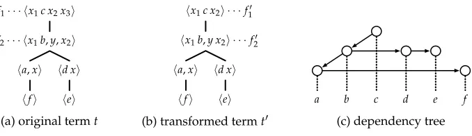
Figure 8
The transformation implemented by the construction of the grammarGin Lemma 4.
f1=x1c x2. To obtainf1 fromf1 wereducethe offending substringx2x3 to the single variablex2. In order to ensure thattandtinduce the same dependency tree (shown in Figure 8c), we thenadaptthe functionf2 =x1b,y,x2at the first child of the root node: Dual to the reduction, we replace the two-component sequencey,x2in the template off2 with the single componenty x2; in this way we getf2=x1b,y x2.
Because adaptation operations may introduce new offending substrings, we need a recursive algorithm to compute the rules of the grammarG. Such an algorithm is given in Table 2. For every ruleA→f(A1,. . .,Am) ofGwe construct new rules
(A,g)→f((A1,g1),. . ., (Am,gm))
wheregand thegiare yield functions encoding adaptation operations. As an example, the adaptation of the functionf2in the termtmay be encoded into the adaptor function x1,x2x3. The functionf2can then be written as the composition of this function andf2:
f2 = x1,x2x3 ◦f2 = x1,x2x3(x1b,y,x2) = x1b,y x2
[image:14.486.56.431.544.671.2]The yield functionfand the adaptor functionsgiare computed based on the template of theg-adapted yield functionf, that is, the composed functiong◦f. In Table 2 we write this asf=reduce(f,g) andgi=adapt(f,g,i), respectively. Let us denote the template of the adapted function g◦f byτ. An i-blockofτis a maximal, non-empty substring of some component ofτthat consists of variables with argument indexi. To compute the template ofgi we read thei-blocks ofτfrom left to right and rename the variables by changing their argument indices fromito 1. To compute the template offwe take the
Table 2
Computing the production rules of an LCFRS in which all yield functions satisfy Property 4.
Input:a linear context-free rewriting systemG=(N,Σ,P,S) 1: P← ∅; agenda← {(S,x)}; chart← ∅
2: whileagendais not empty
3: remove some (A,g) fromagenda
4: if(A,g)∈/chartthen
5: add (A,g) tochart
6: for eachruleA→f(A1,. . .,Am)∈Pdo
7: f←reduce(f,g); gi←adapt(f,g,i) (1≤i≤m)
8: for eachifrom 1 tomdo
9: add (Ai,gi) toagenda
templateτand replace thejthi-block with the variable xi,j, for all argument indicesi and component indicesj.
Our algorithm is controlled by an agenda and a chart, both containing pairs of the form (A,g), where A is a nonterminal of G and g is an adaptor function. These pairs also constitute the nonterminals of the new grammarG. The fan-out of a non-terminal is the fan-out ofg. The agenda is initialized with the pair (S,x) where x is the identity function; this pair also represents the start symbol ofG. To see that the algorithm terminates, one may observe that the fan-out of every nonterminal (A,g) added to the agenda is upper-bounded by the fan-out ofA. Hence, there are only finitely many pairs (A,g) that may occur in the chart, and a finite number of iterations of the while-loop.
We conclude by noting that when constructing a canonical grammar, one needs to be careful about the order in which the individual constructions (for Properties 1–4) are combined. One order that works is
Property 3<Property 4<Property 2<Property 1
6. Parsing and Recognition
Lexicalized linear context-free rewriting systems are able to account for arbitrarily non-projective dependency trees. This expressiveness comes with a price: In this section we show that parsing with lexicalized LCFRSs is intractable, unless we are willing to restrict the class of grammars.
6.1 Parsing Algorithm
To ground our discussion of parsing complexity, we present a simple bottom–up parsing algorithm for LCFRSs, specified as a grammatical deduction system (Shieber, Schabes, and Pereira 1995). Several similar algorithms have been described in the literature (Seki et al. 1991; Bertsch and Nederhof 2001; Kallmeyer 2010). We assume that we are given a grammarG=(N,Σ,P,S) and a stringw=a1· · ·an∈V∗to be parsed.
Item form.The items of the deduction system take the form
[A,l1,r1,. . .,lk,rk]
whereA∈Nwithϕ(A)=k, and the remaining components are indices identifying the left and right endpoints of pairwise non-overlapping substrings ofw. More formally, 0≤lh≤rh≤n, and for all h,h with h=h, either rh≤lh or rh≤lh. The intended interpretation of an item of this form is thatAderives a termt∈T(G) that yields the specified substrings ofw, that is,
A ⇒∗G t and yield(t) = al1+1· · ·ar1,. . .,alk+1· · ·ark
Inference rules.The inference rules of the deduction system are defined based on the rules inP. Each production rule
A→f(A1,. . .,Am) with f :k1· · ·km →k, f =α1,. . .,αk
is converted into a set of inference rules of the form
A1,l1,1,r1,1,. . .,l1,k1,r1,k1
· · · Am,lm,1,rm,1,. . .,lm,km,rm,km
A,l1,r1,. . .,lk,rk
(3)
Each such rule is subject to the following constraints. Let 1≤h≤k,v∈V∗, 1≤i≤m, and 1≤j≤ki. We write δ(l,v)=rto assert thatr=l+|v|and thatv is the substring ofwbetween indiceslandr.
If αh=v then δ(lh,v)=rh (c1)
If v xi,jis a prefix ofαh then δ(lh,v)=li,j (c2)
If xi,jvis a suffix ofαh then δ(ri,j,v)=rh (c3)
If xi,jv xi,jis an infix ofαh then δ(ri,j,v)=li,j (c4)
These constraints ensure that the substrings corresponding to the premises of the inference rule can be combined into the substrings corresponding to the conclusion by means of the yield functionf.
Based on the deduction system, a tabular parser for LCFRSs can be implemented using standard dynamic programming techniques. This parser will compute a packed representation of the set of all derivation trees that the grammar G assigns to the string w. Such a packed representation is often called ashared forest(Lang 1994). In combination with appropriate semirings, the shared forest is useful for many tasks in syntactic analysis and machine learning (Goodman 1999; Li and Eisner 2009).
6.2 Parsing Complexity
We are interested in an upper bound on the runtime of the tabular parser that we have just presented. We can see that the parser runs in timeO(|G||w|c), where|G| denotes the size of some suitable representation of the grammarG, andcdenotes the maximal number of instantiations of an inference rule (cf. McAllester 2002). Let us writec(f) for the specialization ofcto inference rules for productions with yield functionf. We refer to this value as theparsing complexityoff (cf. Gildea 2010). Then to show an upper bound oncit suffices to show an upper bound on the parsing complexities of the yield functions that the parser has to handle. An obvious such upper bound is
c(f) ≤ 2k+ m
i=1 2ki
an upper boundc(f)≤bwe specify a strategy for choosingbendpoints, and then argue that, given the constraints, these choices determine the remaining endpoints.
Lemma 5
For a yield functionf :k1· · ·km→kwe have
c(f) ≤ k+ m
i=1 ki
Proof
We adopt the following strategy for choosing endpoints: For 1≤i≤k, choose the value of lh. Then, for 1≤i≤m and 1≤j≤ki, choose the value of ri,j. It is not hard to see that these choices suffice to determine all other endpoints. In particular, each left endpoint li,j will be shared either with the left endpoint lh of some component (by constraint c2), or with some right endpointri,j(by constraint c4).
6.3 Universal Recognition
The runtime of our parsing algorithm for LCFRSs is exponential in both the rank and the fan-out of the input grammar. One may wonder whether there are parsing algorithms that can be substantially faster. We now show that the answer to this question is likely to be negative even if we restrict ourselves to canonical lexicalized LCFRSs. To this end we study the universal recognition problem for this class of grammars.
The universal recognition problem for a class of linear context-free rewriting systems is to decide, given a grammarG from the class in question and a string w, whetherGyieldsw. A straightforward algorithm for solving this problem is to first compute the shared forest forGand w, and to return “yes” if and only if the shared forest is non-empty. Choosing appropriate data structures, the emptiness of shared forests can be decided in linear time and space with respect to the size of the forest. Therefore, the computational complexity of universal recognition is upper-bounded by the complexity of constructing the shared forest. Conversely, parsing cannot be faster than universal recognition.
In the next three lemmas we prove that the universal recognition problem for canonical lexicalized LCFRSs is NP-complete unless we restrict ourselves to a class of grammars where both the fan-out and the rank of the yield functions are bounded by constants. Lemma 6, which shows that the universal recognition problem of lexicalized LCFRSs is in NP, distinguishes lexicalized LCFRSs from general LCFRSs, for which the universal recognition problem is known to be PSPACE-complete (Kaji et al. 1992). The crucial difference between general and lexicalized LCFRSs is the fact that in the latter, the size of the generated terms is bounded by the length of the input string. Lemma 7 and Lemma 8, which establish two NP-hardness results for lexicalized LCFRSs, are stronger versions of the corresponding results for general LCFRSs presented by Satta (1992), and are proved using similar reductions. They show that the hardness results hold under significant restrictions of the formalism: to lexicalized form and to canonical yield functions. Note that, whereas in Section 5.2 we have shown that every lexicalized LCFRS is equivalent to a canonical one, the normal form transformation increases the size of the original grammar by a factor that is at least exponential in the fan-out.
Lemma 6
Proof
Let Gbe a lexicalized LCFRS, and letwbe a string. To test whether Gyieldsw, we guess a termt∈T(G) and check whethertyieldsw. Let|t|denote the length of some string representation oft. Since the yield functions ofGare lexicalized,|t| ≤ |w||G|. Note that we have
|t| ≤ |w||G| ≤ |w|2+2|w||G|+|G|2 = (|w|+|G|)2
Using a simple tabular algorithm, we can verify in timeO(|w||G|) whether a candidate termtbelongs toT(G). It is then straightforward to compute the string yield oftin time O(|w||G|). Thus we have a nondeterministic polynomial-time decider for the universal recognition problem.
For the following two lemmas, recall the decision problem 3SAT, which is known to be NP-complete. An instance of 3SAT is a Boolean formulaφin conjunctive normal form where each clause contains exactly three literals, which may be either variables or negated variables. We writemfor the number of distinct variables that occur inφ, andn for the number of clauses. In the proofs the indexiwill always range over values from 1 tom, and the indexjwill range over values from 1 ton.
In order to make the grammars in the following reductions more readable, we use yield functions with more than one lexical anchor. Our use of these yield functions is severely restricted, however, and each of our grammars can be transformed into a proper lexicalized LCFRS without affecting the correctness or polynomial size of the reductions.
Lemma 7
The universal recognition problem for canonical lexicalized LCFRSs with unbounded fan-out and rank 1 is NP-hard.
Proof
To prove this claim, we provide a polynomial-time reduction of 3SAT. The basic idea is to use the derivations of the grammar to guess truth assignments for the variables, and to use the feature of unbounded fan-out to ensure that the truth assignment satisfies all clauses.
Letφbe an instance of 3SAT. We construct a canonical lexicalized LCFRSGand a string was follows. Let Mdenote them×nmatrix with entriesMi,j=(vi,cj), that is, entries in the same row share the same variable, and entries in the same column share the same clause. We set upGin such a way that each of its derivations simulates a row-wise iteration overM. Before visiting a new row, the derivation chooses a truth value for the corresponding variable, and sticks to that choice until the end of the row. The stringwtakes the form
w = w1$· · ·$wn where wj = cj,1· · ·cj,mcj,1· · ·cj,m
This string is built up during the iteration overMin a column-wise fashion, where each column corresponds to one component of a tuple with fan-outn. More specifically, for each entry (vi,cj), the derivation generates one of two strings, denoted byγi,jand ¯γi,j:
The stringγi,j is generated only ifvican be used to satisfy cj under the hypothesized truth assignment. By this construction, every successful derivation ofGrepresents a truth assignment that satisfiesφ. Conversely, using a satisfying truth assignment forφ, we will be able to construct a derivation ofGthat yieldsw.
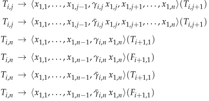
To see how the traversal of the matrixMcan be implemented by the grammarG, consider the grammar fragment in Figure 9. Each of the rules specifies one possible step of the iteration for the pair (vi,cj) under the truth assignmentvi=true; rules with left-hand sideFi,j(not shown here) specify possible steps under the assignmentvi=false.
Lemma 8
The universal recognition problem for canonical lexicalized LCFRSs with unbounded rank and fan-out 2 is NP-hard.
Proof
We provide another polynomial-time reduction of 3SAT to a grammarGand a stringw, again based on the matrixMmentioned in the previous proof. Also as in the previous reduction, we set up the grammarGto simulate a row-wise iteration overM. The major difference this time is that the entries of M are not visited during one long rank 1 derivation, but duringmnrather short fan-out 2 subderivations. The stringwis
w = w,1· · ·w,m$w,1· · ·w,n
where w,i = ai,1· · ·ai,nbi,1· · ·bi,n and w,j = c1,j· · ·cm,jc1,j· · ·cm,j
During the traversal ofM, for each entry (vi,cj), we generate a tuple consisting of two substrings ofw. The right component of the tuple consists of one the two stringsγi,j and ¯γi,j mentioned previously. As before, the string γi,j is generated only ifvi can be used to satisfycjunder the hypothesized truth assignment. The left component consists of one of two strings, denoted byσi,jand ¯σi,j:
σi,1=ai,1· · ·ai,nbi,1 σi,j=bi,j (1<j) σ¯i,n=ai,nbi,1· · ·bi,n σ¯i,j=ai,j (j<n)
[image:19.486.53.269.531.635.2]These strings are generated to represent the truth assignmentsvi=trueandvi=false, respectively. By this construction, each substringw,i can be derived in exactly one of two ways, ensuring a consistent truth assignment for all subderivations that are linked to the same variablevi.
Figure 9
The grammarGis defined as follows. There is one rather complex rule to rewrite the start symbolS; this rule sets up the general topology ofw. LetIbe them×nmatrix with entriesIi,j=(j−1)m+i. Definex1to be the sequence of variables of the formxh,1, where the argument indexiis taken from a row-wise reading of the matrixI; in this case, the argument indices inxwill simply go up from 1 tomn. Now definex2to be the sequence of variables of the formxh,2, wherehis taken from a column-wise reading of the matrixI. ThenScan be expanded with the rule
S → x1$x2(V1,1,. . .,V1,n,. . .,Vm,1,. . .,Vm,n)
Note that there is one nonterminalVi,j for each variable–clause pair (vi,cj). These non-terminals can be rewritten using the following rules:
Vi,1 → σi,1,x(Ti,1) Vi,j → σi,j,x(Ti,j)
Vi,n → σ¯i,n,x(Fi,n) Vi,j → σ¯i,j,x(Fi,j)
The remaining rules rewrite the nonterminalsTi,jandFi,j:
Ti,j → γi,j (ifvioccurs incj) Ti,j → γ¯i,j
Fi,j → γi,j (if ¯vioccurs incj) Fi,j → γ¯i,j
It is not hard to see that bothGandwcan be constructed in polynomial time.
7. Block-Degree
To obtain efficient parsing, we would like to have grammars with as low a fan-out as possible. Therefore it is interesting to know how low we can go without losing too much coverage. In lexicalized LCFRSs extracted from dependency treebanks, the fan-out of a grammar has a structural correspondence in the maximal number of blocks per subtree, a measure known as “block-degree.” In this section we formally define block-degree, and evaluate grammar coverage under different bounds on this measure.
7.1 Definition of Block-Degree
Recall the concept of “blocks” that was defined in Section 4.2. The block-degreeof a nodeuof a dependency treeDis the number of distinct blocks ofu. The block-degree ofDis the maximal block-degree of its nodes.2
Example 6
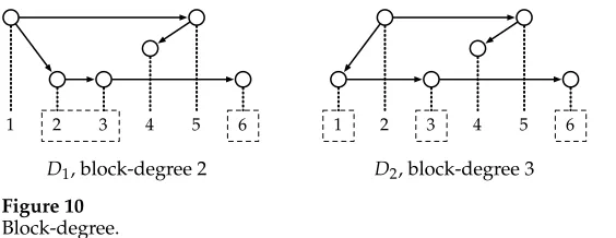
Figure 10 shows two non-projective dependency trees. ForD1, consider the node 2. The descendants of 2 fall into two blocks, marked by the dashed boxes. Because this is the maximal number of blocks per node inD1, the block-degree ofD1is 2. Similarly, we can verify that the block-degree of the dependency treeD2is 3.
Figure 10
Block-degree.
A dependency tree isprojectiveif its block-degree is 1. In a projective dependency tree, each subtree corresponds to a substring of the underlying tuple of strings. In a non-projective dependency tree, a subtree may span over several, discontinuous substrings.
7.2 Computing the Block-Degrees
Using a straightforward extension of the algorithm in Table 1, the block-degrees of all nodes of a dependency tree Dcan be computed in time O(m), where mis the total number of blocks. To compute the block-degree ofD, we simply take the maximum over the degrees of each node. We can also adapt this procedure to test whetherDis projective, by aborting the computation as soon as we discover that some node has more than one block. The runtime of this test is linear in the number of nodes ofD.
7.3 Block-Degree in Extracted Grammars
In a lexicalized LCFRS extracted from a dependency treebank, there is a one-to-one correspondence between the blocks of a nodeu and the components of the template of the yield function f extracted for u. In particular, the fan-out of f is exactly the block-degree of u. As a consequence, any bound on the block-degree of the trees in the treebank translates into a bound on the fan-out of the extracted grammar. This has consequences for the generative capacity of the grammars: As Seki et al. (1991) show, the class of LCFRSs with fan-outk>1 can generate string languages that cannot be generated by the class of LCFRSs with fan-outk−1.
It may be worth emphasizing that the one-to-one correspondence between blocks and tuple components is a consequence of two characteristic properties of extracted grammars (Properties 3 and 4), and does not hold for non-canonical lexicalized LCFRSs.
Example 7
The following term induces a two-node dependency tree with block-degree 1, but contains yield functions with fan-out 2:a x1x2(b,ε). Note that the yield functions in this term violate both Property 3 and Property 4.
7.4 Coverage on Dependency Treebanks
dependency treebanks used in the 2006 CoNLL shared task on dependency parsing (Buchholz and Marsi 2006): the Prague Arabic Dependency Treebank (Hajiˇc et al. 2004), the Prague Dependency Treebank of Czech (B ¨ohmov´a et al. 2003), the Danish Depen-dency Treebank (Kromann 2003), the Slovene DepenDepen-dency Treebank (Dˇzeroski et al. 2006), and the Metu-Sabancı treebank of Turkish (Oflazer et al. 2003). The full data used in the CoNLL shared task also included treebanks that were produced by conversion of corpora originally annotated with structures other than dependencies, which is a potential source of “noise” that one has to take into account when interpreting any findings. Here, we consider only genuine dependency treebanks. More specifically, our statistics concern the training sections of the treebanks that were set off for the task. For similar results on other data sets, see Kuhlmann and Nivre (2006), Havelka (2007), and Maier and Lichte (2011).
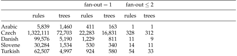
Our results are given in Table 3. For each treebank, we list the number of rules extracted from that treebank, as well as the number of corresponding dependency trees. We then list the number of rules that we lose if we restrict ourselves to rules with fan-out=1, or rules with fan-out≤2, as well as the number of dependency trees that we lose because their construction trees contain at least one such rule. We count ruletokens, meaning that two otherwise identical rules are counted twice if they were extracted from different trees, or from different nodes in the same tree.
By putting the bound at fan-out 1, we lose between 0.74% (Arabic) and 1.75% (Slovene) of the rules, and between 11.16% (Arabic) and 23.15% (Czech) of the trees in the treebanks. This loss is quite substantial. If we instead put the bound at fan-out ≤ 2, then rule loss is reduced by between 94.16% (Turkish) and 99.76% (Arabic), and tree loss is reduced by between 94.31% (Turkish) and 99.39% (Arabic). This outcome is surprising. For example, Holan et al. (1998) argue that it is impossible to give a theoretical upper bound for the block-degree of reasonable dependency analyses of Czech. Here we find that, if we are ready to accept a loss of as little as 0.02% of the rules extracted from the Prague Dependency Treebank, and up to 0.5% of the trees, then such an upper bound can be set at a block-degree as low as 2.
8. Well-Nestedness
[image:22.486.48.434.571.662.2]The parsing of LCFRSs is exponential both in the fan-out and in the rank of the grammars. In this section we study “well-nestedness,” another restriction on the non-projectivity of dependency trees, and show how enforcing this constraint allows us to restrict our attention to the class of LCFRSs with rank 2.
Table 3
Loss in coverage under the restriction to yield functions with fan-out=1 and fan-out≤2.
fan-out=1 fan-out≤2
rules trees rules trees rules trees
Arabic 5,839 1,460 411 163 1 1
Czech 1,322,111 72,703 22,283 16,831 328 312
Danish 99,576 5,190 1,229 811 11 9
Slovene 30,284 1,534 530 340 14 11
8.1 Definition of Well-Nestedness
Let D be a dependency tree, and let u and v be nodes of D. The descendants of u and v overlap, denoted by uv, if there exist nodes ul,ur∈ u and vl,vr∈ v such that
ul<vl<ur <vr or vl<ul<vr<ur
A dependency treeDis calledwell-nestedif for all pairs of nodesu,vofD
uv implies that u ∩ v =∅
In other words,uandvmay overlap only ifuis an ancestor ofv, orvis an ancestor ofu. If this implication does not hold, thenDis calledill-nested.
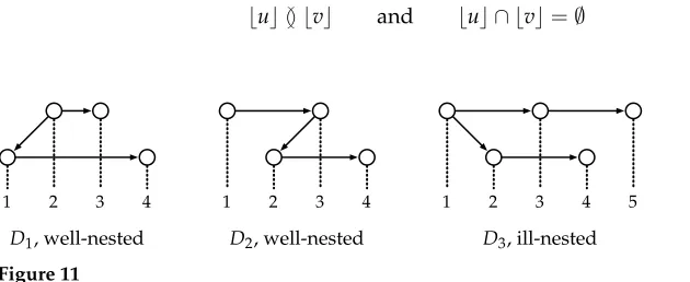
Example 8
Figure 11 shows three non-projective dependency trees. BothD1andD2are well-nested: D1 does not contain any overlapping sets of descendants at all. In D2, although 1 and2overlap, it is also the case that1 ⊇ 2. In contrast,D3is ill-nested, as
23 but 2 ∩ 3=∅
The following lemma characterizes well-nestedness in terms of blocks.
Lemma 9
A dependency tree is ill-nested if and only if it contains two sibling nodesu,vand blocks u1,u2ofuandv1,v2ofvsuch that
u1<v1<u2<v2 (4)
Proof
LetDbe a dependency tree. Suppose thatDcontains a configuration of the form (4). This configuration witnesses that the setsuandvoverlap. Becauseu,vare siblings, u ∩ v=∅. Therefore we conclude that D is ill-nested. Conversely now, suppose thatDis ill-nested. In this case, there exist two nodesuandvsuch that
[image:23.486.55.370.519.648.2]uv and u ∩ v=∅ (∗)
Figure 11
Here, we may assumeuandv to be siblings: otherwise, we may replace eitheruorv with its parent node, and property (∗) will continue to hold. Becauseuv, there exist descendantsul,ur∈ uandvl,vr∈ vsuch that
ul<vl<ur<vr or vl<ul<vr<ur
Without loss of generality, assume that we have the first case. The nodesulandurbelong to different blocks ofu, sayu1andu2; and the nodesvlandvrbelong to different blocks ofv, sayv1andv2. Then it is not hard to verify Equation (4).
Note that projective dependency trees are always well-nested; in these structures, every node has exactly one block, so configuration (4) is impossible. For every k>1, there are both well-nested and ill-nested dependency trees with block-degreek.
8.2 Testing for Well-Nestedness
Based on Lemma 9, testing whether a dependency treeDis well-nested can be done in time linear in the number of blocks inDusing a simple subsequence test as follows. We run the algorithm given in Table 1, maintaining a stacks[u] for every nodeu. The first time we make a down step tou, we pushuto the stack for the parent ofu; every other time, we pop the stack for the parent until we either finduas the topmost element, or the stack becomes empty. In the latter case, we terminate the computation and report thatD is ill-nested; if the computation can be completed without any stack ever becoming empty, we report thatDis well-nested.
To show that the algorithm is sound, suppose that some stacks[p] becomes empty when making a down step to some childvofp. In this case, the nodevmust have been popped froms[p] when making a down step to some other childuofp, and that child must have already been on the stack before the first down step tov. This witnesses the existence of a configuration of the form in Equation (4).
8.3 Well-Nestedness in Extracted Grammars
Just like block-degree, well-nestedness can be characterized in terms of yield functions. Recall the notationx<f yfrom Section 5.1. A yield function
f :k1· · ·km→k, f =α1,. . .,αk
is ill-nested if there are argument indices 1≤i1,i2≤m with i1=i2 and component indices 1≤j1,j1 ≤ki1, 1≤j2,j
2≤ki2such that
xi1,j1 <f xi2,j2 <f xi1,j1 <f xi2,j2 (5)
Otherwise, we say thatf iswell-nested. As an immediate consequence of Lemma 9, a restriction to well-nested dependency trees translates into a restriction to well-nested yield functions in the extracted grammars. This puts them into the class of what Kanazawa (2009) calls “well-nested multiple context-free grammars.”3These grammars
have a number of interesting properties that set them apart from general LCFRSs; in particular, they have a standard pumping lemma (Kanazawa 2009). The yield languages generated by well-nested multiple context-free grammars form a proper subhierarchy within the languages generated by general LCFRSs (Kanazawa and Salvati 2010). Per-haps the most prominent subclass of well-nested LCFRSs is the class of tree-adjoining grammars (Joshi and Schabes 1997).
Similar to the situation with block-degree, the correspondence between structural well-nestedness and syntactic well-nestedness is tight only for canonical grammars. For non-canonical grammars, syntactic well-nestedness alone does not imply structural well-nestedness, nor the other way around.
8.4 Coverage on Dependency Treebanks
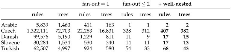
To estimate the coverage of well-nested grammars, we extend the evaluation presented in Section 7.4. Table 4 shows how many rules and trees in the five dependency treebanks we lose if we restrict ourselves to well-nested yield functions with fan-out≤ 2. The losses reported in Table 3 are repeated here for comparison. Although the coverage of well-nested rules is significantly smaller than the coverage of rules without this requirement, rule loss is still reduced by between 92.65% (Turkish) and 99.51% (Arabic) when compared to the fan-out=1 baseline.
8.5 Binarization of Well-Nested Grammars
Our main interest in well-nestedness comes from the following:
Lemma 10
The universal recognition problem for well-nested lexicalized LCFRS with fan-outkand unbounded rank can be decided in time
O
|G| · |w|2k+2
[image:25.486.52.438.572.662.2]To prove this lemma, we will provide an algorithm for thebinarization of well-nested lexicalized LCFRSs. In the context of LCFRSs, a binarization is a procedure for transforming a grammar into an equivalent one with rank at most 2. Binarization, either explicit at the level or the grammar or implicit at the level of some parsing algorithm, is essential for achieving efficient recognition algorithms, in particular the usual cubic-time algorithms for context-free grammars. Note that our binarization only
Table 4
Loss in coverage under the restriction to yield functions with fan-out=1, fan-out≤2, and to well-nested yield functions with fan-out≤2 (last column).
fan-out=1 fan-out≤2 + well-nested
rules trees rules trees rules trees rules trees
Arabic 5,839 1,460 411 163 1 1 2 2
Czech 1,322,111 72,703 22,283 16,831 328 312 407 382
Danish 99,576 5,190 1,229 811 11 9 17 15
Slovene 30,284 1,534 530 340 14 11 17 13
preservesweakequivalence; in effect, it reduces the universal recognition problem for well-nested lexicalized LCFRSs to the corresponding problem for well-nested LCFRSs with rank 2. Many interesting semiring computations on the original grammar can be simulated on the binarized grammar, however. A direct parsing algorithm for well-nested dependency trees has been presented by G ´omez-Rodr´ıguez, Carroll, and Weir (2011).
The binarization that we present here is a special case of the binarization proposed by G ´omez-Rodr´ıguez, Kuhlmann, and Satta (2010). They show that every well-nested LCFRS can be transformed (at the cost of a linear size increase) into a weakly equivalent one in which all yield functions are either constants (that is, have rank 0) or binary functions of one of two types:
x1,. . .,xk1y1,. . .,yk2:k1k2 →(k1+k2−1) (concatenation) (6)
x1,. . .,xjy1,. . .,yk2xj+1,. . .,xk1:k1k2 →(k1+k2−2) (wrapping) (7)
Aconcatenation functiontakes ak1-tuple and ak2-tuple and returns the (k1+k2− 1)-tuple that is obtained by concatenating the two arguments. The simplest concatenation function is the standard concatenation operationx y. We will writeconc:k1k2 to refer to a concatenation function of the type given in Equation (6). By counting endpoints, we see that the parsing complexity of concatenation functions is
c(conc:k1k2) ≤ 2k1+2k2−1
Awrapping functiontakes ak1-tuple (for somek1≥2) and ak2-tuple and returns the (k1+k2−2)-tuple that is obtained by “wrapping” the first argument around the second argument, filling some gap in the former. The simplest function of this type isx1y x2, which wraps a 2-tuple around a 1-tuple. We write wrap:k1k2jto refer to a wrapping function of the type given in Equation (7). The parsing complexity is
c(wrap:k1k2j) ≤ 2k1+2k2−2 (for all choices ofj)
The constants of the binarized grammar have the formε,ε,ε, anda, whereais the anchor of some yield function of the original grammar.
8.5.1 Parsing Complexity.Before presenting the actual binarization, we determine the parsing complexity of the binarized grammar. Because the binarization preserves the fan-out of the original grammar, and because in a grammar with fan-outk, for con-catenation functions conc:k1k2 we have k1+k2−1≤k and for wrapping functions wrap:k1k2jwe havek1+k2−2≤k, we can rewrite the general parsing complexities as
c(conc:k1k2) ≤ 2k1+2k2−1 = 2(k1+k2−1)+1 ≤ 2k+1
c(wrap:k1k2j) ≤ 2k1+2k2−2 = 2(k1+k2−2)+2 ≤ 2k+2
Figure 12
Binarization of well-nested LCFRSs (complex cases).
8.5.2 Binarization.We now turn to the actual binarization. Consider a rule
A→f(A1,. . .,Am)
wheref is not already a concatenation function, wrapping function, or constant. We decompose this rule into up to three rules
A→f(B,C) B→f1(B1,. . .,Bm1) C→f2(C1,. . .,Cm2)
as follows. We match the template off against one of three cases, shown schematically in Figure 12. In each case we select a concatenation or wrapping functionf(shown in the right half of the figure), and split up the template off into two parts defining yield functionsf1andf2, respectively. In Figure 12,f1 is drawn shaded, andf2is drawn non-shaded.4 The split off partitions the variables that occur in the template, in the sense
that if for some argument index 1≤i≤m, eitherf1 or f2 contains any variable with argument indexi, then it containsallsuch variables. The two sequences
B1,. . .,Bm1 and C1,. . .,Cm2 are obtained from A1,. . .,Am
by collecting the nonterminal Ai if the variables with argument index ibelong to the template off1andf2, respectively. The nonterminalsBandCare fresh nonterminals. We do not create rules forf1andf2if they are identity functions.
Example 9
We illustrate the binarization by showing how to transform the rule
A→ x1a x2y1,y2,y3x3(A1,A2)
The templatex1a x2y1,y2,y3x3is complex and matches Case 3 in Figure 12, because its first component starts with the variable x1 and its last component ends with the variable x3. We therefore split the template into two smaller parts x1a x2,x3 and y1,y2,y3. The functiony1,y2,y3is an identity. We therefore create two rules:
A→f1(X,A2) , f1=wrap: 2 3 1=x1y1,y2,y3x2 X→ x1a x2,x3(A1)
Note that the index jfor the wrapping function was chosen to bej=2 because there were more component boundaries between x2 and x3 than between x1 and x2. The templatex1a x2,x3requires further decomposition according to Case 3. This time, the two smaller parts are the identity functionx1,x2,x3and the constanta. We therefore create the following rules:
X→f2(A1,Y) , f2=wrap: 3 1 1=x1y x2,x3 Y→ a
At this point, the transformation ends.
8.5.3 Correctness.We need to show that the fan-out of the binarized grammar does not exceed the fan-out of the original grammar. We reason as follows. Starting from some initial yield function f0 :k1· · ·km→k, each step of the binarization decomposes some yield function f into two new yield functionsf1,f2. Let us denote the fan-outs of the three functions byh,h1,h2, respectively. We have
h = h1+h2−1 in Case 1 and Case 2 (8)
h = h1+h2−2 in Case 3 (9)