Lexical Tightness and Text Complexity
Michael Flor
Beata Beigman Klebanov
Kathleen M. Sheehan
Educational Testing Service Princeton, NJ, 08541, USA
{mflor,bbeigmanklebanov,ksheehan}@ets.org
Abstract
We present a computational notion of Lexical Tightness that measures global cohesion of con-tent words in a text. Lexical tightness represents the degree to which a text tends to use words that are highly inter-associated in the language. We demonstrate the utility of this measure for estimating text complexity as measured by US school grade level designations of texts. Lexical tightness strongly correlates with grade level in a collection of expertly rated reading materials. Lexical tightness captures aspects of prose complexity that are not covered by classic read-ability indexes, especially for literary texts. We also present initial findings on the utility of this measure for automated estimation of complex-ity for poetry.
1 Introduction
Adequate estimation of text complexity has a long and rich history. Various readability metrics have been designed in the last 100 years (DuBay, 2004). Recent work on computational estimation of text complexity for school- and college-level texts in-cludes (Vajjala and Meurers 2012; Graesser et al., 2011; Sheehan et al., 2010; Petersen and Osten-dorf, 2009; Heilman et al., 2006). Several commer-cial systems were recently evaluated in the Race To The Top competition (Nelson et al., 2012) in relation to the US Common Core State Standards for instruction (CCSSI, 2010).
A variety of factors influence text complexity, including vocabulary, sentence structure, academic orientation, narrativity, cohesion, etc. (Hiebert,
2011) and corresponding features are utilized in automated systems of complexity evaluation (Vajjala and Meurers, 2012; Graesser et al., 2011; Sheehan et al., 2010).
We focus on text complexity levels expressed as US school grade level equivalents1. Our interest is
in quantifying the differences among texts (es-say-length reading passages) at different grade levels, for the purposes of automatically evaluating text complexity. The work described in this paper is part of an ongoing project that investigates novel features indicative of text complexity.
The paper is organized as follows. Section 2.1 presents our methodology for building word asso-ciation profiles for texts. Section 2.2 defines the measure of lexical tightness (LT). Section 2.3 de-scribes the datasets used in this study. Sections 3.1 and 3.2 present our study of the relationship between LT and text complexity. Section 3.3 de-scribes application to poetry. Section 3.4 evaluates an improved measure (LTR). Section 4 reviews re-lated work.
2 Methodology
2.1 Word-Association Profile
We define WAPT – a word association profile of a
text T – as the distribution of association values for all pairs of content words of text T, where the asso-ciation values are estimated from a very large cor-pus of texts. In this work, WAP is purely illustrat-ive, and sets the stage for lexical tightness.
1 For age equivalents of grade levels see
http://en.wikipedia.org/wiki/Educational_stage
There exists an extensive literature on the use of word-association measures for NLP, especially for detection of collocations (Pecina, 2010; Evert, 2008). The use of pointwise mutual information (PMI) with word-space models is noted in (Zhang et al., 2012; Baroni and Lenci, 2010; Mitchell and Lapata, 2008; Turney, 2001). We begin with PMI, and provide a modified measure in later sections.
To obtain comprehensive information about co-occurrence behavior of words in English, we build a first-order co-occurrence word-space model (Turney and Pantel, 2010; Baroni and Lenci, 2010). The model was generated from a corpus of texts of about 2.5 billion word tokens, counting non-directed co-occurrence in a paragraph, using no distance coefficients (Bullinaria and Levy, 2007). About 2 billion word tokens come from the Gigaword 2003 corpus (Graff and Cieri, 2003). Additional 500 million word tokens come from an in-house corpus containing texts from the genres of fiction and popular science. The matrix of 2.1x2.1 million word types and their co-occurrence fre-quencies, as well as single-word frefre-quencies, is ef-ficiently compressed using the TrendStream tech-nology (Flor, 2013), resulting in a database file of 4.7GB. The same toolkit allows fast retrieval of word probabilities and statistical associations for pairs of words.2
In this study we use all content word tokens of a text. We use the OpenNLP tagger3 to POS-tag a
text and only take into account nouns, verbs, ad-jective and adverbs. We further apply a stop-list (see Appendix A) to filter out auxiliary verbs.
To illustrate why WAP is an interesting notion, consider this toy example: The texts “The dog barked and wagged its tail” vs. “Green ideas sleep furiously”. Their matrices of pairwise word associ-ations are presented in Table 1. For the first text, all the six content word pairs score above PMI=5.5. On the other hand, for “Green ideas sleep furiously”, all the six content word pairs score below PMI=2.2. The first text puts together words that often go together in English, and this
might be one of the reasons it seems easier to un-derstand than the second text.
We use histograms to illustrate word-association profiles for real texts, containing hundreds of
2 The distributional word-space model includes counts for 2.1
million words and 1279 million word pairs (types). Associ-ation measures are computed on the fly.
3http://opennlp.apache.org
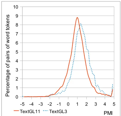
words. For a 60-bin histrogram spanning all ob-tained PMI values, the lowest bin contains pairs with PMI≤–5, the highest bin contains pairs with PMI>4.83, while the rest of the bins contain word pairs (a,b) with -5<PMI(a,b)≤4.83. Figure 1 presents WAP histograms for two real text samples, one for grade level 3 (age 8-9) and one for grade level 11 (age 16-17). We observe that the shape of distribution is normal-like. The distribu-tion of GL3 text is shifted to the right – it contains more highly associated word-pairs than the text of GL11. In a separate study we investigated the properties of WAP distribution (Beigman-Kleban-ov and Flor, 2013). The normal-like shape turns out to be stable across a variety of texts.
The dog barked and wagged its tail:
dog barked wagged tail
dog 7.02 7.64 5.57
barked 9.18 5.95
wagged 9.45
tail
Green ideas sleep furiously:
green ideas sleep furiously
green 0.44 1.47 2.05
ideas 1.01 0.94
sleep 2.18
[image:2.612.319.535.258.400.2]furiously
Table 1. Word association matrices (PMI values) for two illustrative examples.
-5 -4 -3 -2 -1 0 1 2 3 4 5 0
1 2 3 4 5 6 7 8 9 10
TextGL11 TextGL3 PMI
P
e
rc
e
n
ta
g
e
o
f p
a
ir
s
o
f w
o
rd
to
ke
n
s
[image:2.612.322.530.439.639.2]2.2 Lexical Tightness
In this section we consider how to derive a single measure to represent each text for further analyses. Given the stable normal-like shape of WAP, we use average (mean) value per text for further in-vestigations. We experimented with several associ-ation measures.
Point-wise mutual information is defined as fol-lows (Church and Hanks, 1990):
PMI =
log
2p
a ,b
p
a
p
b
Normalized PMI (Bouma, 2009):
NPMI = 2 2
( , )
log
log
( , )
( ) ( )
p a b
p a b
p a p b
−
Unlike the standard PMI (Manning and Schütze, 1999), NPMI has the property that its values are mostly constrained in the range {-1,1}, it is less in-fluenced by rare extreme values, which is conveni-ent for summing values over multiple pairs of words. Additional experiments on our data have shown that ignoring negative NPMI values4. works
best. Thus, we define Positive Normalized PMI (PNPMI) for a pair of words a and b as follows:
PNPMI(a,b)
= NPMI(a,b) if NPMI(a,b)>0 = 0 if NPMI(a,b)≤0
or if database has no data for co-occurrence of a and b.5
We define Lexical Tightness (LT) of a text as the mean value of PNPMI for all pairs of content-word tokens in a text. Thus, if a text has N words, and after filtering we remain with K content words, the total number of pairs is K*(K-1)/2.
Lexical tightness represents the degree to which a text tends to use words that are highly inter-asso-ciated in the language. We conjecture that lexically tight texts (with higher values of LT) are easier to read and would thus correspond to lower grade levels.
4 Ignoring negative values is described by Bullinaria and Levy
(2007), also Mohammad and Hirst (2006).
5In our text collection, the average percentage of word-pairs
not found in database is 5.5% per text.
2.3 Datasets
Our data consists of two sets of passages. The first set consists of 1012 passages (636K words) – read-ing materials that were used in various tests in state and national assessment frameworks in the USA. Part of this set is taken from Sheehan et al. (2007) (from testing programs and US state departments of education), and part was taken from the Standar-dized State Test Passages set of the Race To The Top (RTT) competition (Nelson et al., 2012). A distinguishing feature of this dataset is that the ex-act grade level specification was available for each text. Table 2 provides the breakdown by grade and genre. Text length in this set ranged between 27 and 2848 words, with average 629 words. Average text length in the literary subset was 689 words and in the informational subset 560 words.
Grade
Level Inf GenreLit Other Total
1 2 4 1 7
2 2 4 3 9
3 49 63 10 122
4 54 77 8 139
5 47 48 15 110
6 44 43 6 93
7 39 61 6 106
8 73 66 19 158
9 25 25 3 53
10 29 52 2 83
11 18 25 0 43
12 47 20 22 89
[image:3.612.312.542.304.479.2]Total 429 488 95 1012
Table 2. Counts of texts by grade level and genre, set #1
Grade
Band GL Inf GenreLit Other Total
2–3 2.5 6 10 4 20
4–5 4.5 16 10 4 30
6–8 7 12 16 13 41
9–10 9.5 12 10 17 39
11+ ' 11.5 8 10 20 38
Total 54 56 58 168
Table 3. Counts of texts by grade band and genre, for dataset #2. GL specifies our grade level designation.
The second dataset comprises 168 texts (80.8K word tokens) from Appendix B of the Common Core State Standards (CCSSI, 2010)6, not
ing poetry items. Exact grade level designations are not available for this set, rather the texts are classified into grade bands, as established by ex-pert instructors (Nelson et al., 2012). Table 3 provides the breakdown by grade and genre. Text length in this set ranged between 99 and 2073 words, with average 481 words. Average text length in the literary subset was 455 words and in the informational subset 373 words.
Our collection is not very large in terms of typical datasets used in NLP research. However, it has two unique facets: grading and genres. Rather than having grade-ranges, set #1 has exact grade designations for each text. Moreover, these were rated by educational experts and used in state and nationwide testing programs.
Previous research has emphasized the importan-ce of genre effects for predicting readability and complexity (Sheehan et al., 2008) and for text ad-aptation (Fountas and Pinnell, 2001). For all texts in our collection, genre designations (information-al, literary, or 'other') were provided by expert hu-man judges (we used the designations that were prepared for the RTT competition, Nelson et al., 2012). The 'other' category included texts that were somewhere in between literary and informational (e.g. biographies), as well as speeches, schedules, and manuals.
3 Results
3.1 Lexical Tightness and Grade Level
Correlations of lexical tightness with grade level are shown in Table 4, for sets 1 and 2, the com-bined set and for literary and informational subsets. Our first finding is that lexical tightness has con-siderable and statistically significant correlation with grade level, in each dataset, in the combined dataset and for the specific subsets. Notably the correlation between lexical tightness and grade level is negative. Texts of higher grade levels are lexically less tight, as predicted.
Although in these datasets grade level is mode-rately correlated with text length, lexical tightness remains considerably and significantly correlated with grade level even after removing the influence of correlations with text length.
Our second finding is that lexical tightness has a stronger correlation with grade level for the subset of literary texts (r=-0.610) than for informational
texts (r=-0.499) in set #1. A similar pattern exists for set #2.
Figure 2 shows the average LT for each grade level, for texts of set #1. As the grade level in-creases, average lexical tightness values decrease consistently, especially for informational and liter-ary texts. There are two 'outliers'. Informational texts for grade 12 show a sudden increase in lexic-al tightness. Also, for genre 'other', grades 9,10,11 are underepresented (see Table 2).
Subset N GL&lengthCorrelation Correlation GL<
Partial Correlation
GL< Set #1
All 1012 0.362 -0.546 -0.472
Inf 429 0.396 -0.499 -0.404
Lit 488 0.408 -0.610 -0.549
Set #2 (Common Core)
All 168 0.360 -0.441 -0.373
Inf 54 0.406 -0.313 -0.347
Lit 56 0.251 -0.546 -0.505
Combined set
All 1180 0.339 -0.528 -0.462
Inf 483 0.386 -0.472 -0.369
Lit 544 0.374 -0.601 -0.545
Table 4. Correlations of grade level (GL) with text length and lexical tightness (LT). Partial correlation GL< controls for text length. All correlations are significant with p<0.04.
Figure 3 shows the average LT for each grade band, for texts of set #2. Here as well, decrease of lexical tightness is evident with increase of grade
3 4 5 6 7 8 9 10 11 12 0.040
0.045 0.050 0.055 0.060 0.065 0.070
Lexical Tightness by Grade Level
Inf Lit other
Grade Level
L
e
xi
ca
l T
ig
h
tn
e
s
[image:4.612.316.538.432.618.2]s
level. In this small set, informational texts show a relatively smooth decrease of LT, while literary texts show a sharp decrease of LT in transition from grade band 4-5 (4.5) to grade band 6-8 (7). Texts labelled as 'other' genre in set #2 are gener-ally less 'tight' than literary or informational. Also for 'other' genre, bands 7-8, 9-10 and 11-12 have equal lexical tighness.
3.2 Grade Level and Readability Indexes
We have also calculated readability indexes for each passage in sets 1 and 2. We used well known readability formulae: Flesch-Kincaid Grade Level (FKGL: Kincaid et al., 1975), Flesch Reading Ease (FRE: Flesch, 1948), Gunning-Fog Index (GFI: Gunning, 19527), Coleman Liau Index (CLI:
Cole-man and Liau, 1975) and Automated Readability Index (ARI: Senter and Smith, 1967). All of them are based on measuring the length of words (in let-ters or syllables) and length of sentences (mean number of words). For our collection, we also computed the average sentence length (avgSL, as word count), average word frequency8 (avgWF –
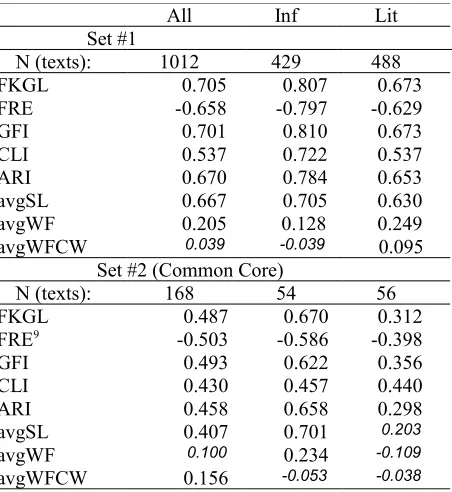
over all words), and average word frequency for only content words (avgWFCW). Results are shown in Table 5.
Word frequency has quite low correlation with grade level in both datasets. Readability indexes
7 Using the modern formula, as referenced at
http://en.wikipe-dia.org/wiki/Fog_Index
8 For word frequency we use the unigrams data from the
Google Web1T collection (Brants and Franz, 2006).
have a strong and consistent correlation with grade level. For dataset #1, readability indexes have much stronger correlation with grade level for in-formational texts (|r| between 0.7 and 0.81) as compared to literary texts (|r| between 0.53 and 0.68), and a similar pattern is seen for dataset #2, with overall lower correlation.
The correlation of Flesch-Kincaid (FKGL) val-ues with LT are r=-0.444 for set #1, r=-0.499 for the informational subset and r=-0.541 for literary subset. The correlation is r=-0.182 in set #2.
All Inf Lit
Set #1
N (texts): 1012 429 488
FKGL 0.705 0.807 0.673
FRE -0.658 -0.797 -0.629
GFI 0.701 0.810 0.673
CLI 0.537 0.722 0.537
ARI 0.670 0.784 0.653
avgSL 0.667 0.705 0.630
avgWF 0.205 0.128 0.249
avgWFCW 0.039 -0.039 0.095
Set #2 (Common Core)
N (texts): 168 54 56
FKGL 0.487 0.670 0.312
FRE9 -0.503 -0.586 -0.398
GFI 0.493 0.622 0.356
CLI 0.430 0.457 0.440
ARI 0.458 0.658 0.298
avgSL 0.407 0.701 0.203
avgWF 0.100 0.234 -0.109
[image:5.612.74.297.172.360.2]avgWFCW 0.156 -0.053 -0.038
Table 5. Correlations of grade level with readability formulae and word frequency. All correlations apart from the italicized ones are significant with p<0.05. Abbreviations are explained in the text.
3.3 Lexical Tightness and Readability Indexes
To evaluate the usefulness of LT in predicting grade level of passages, we estimate, using dataset #1, a linear regression model where the grade level is a dependent variable and Flesch-Kincaid score and lexical tightness are the two independent vari-ables (features). First, we checked whether regres-sion model improves over FKGL in the training set (#1). Then, we tested the regression model estim-ated on 1012 texts of set #1, on 168 texts of set #2.
The results of the regression model on 1012 texts of set #1 (R2=0.565, F(2,1009)=655.85,
9 Flesch Reading Ease formula is inversely related to grade
level, hence the negative correlations.
2.5 4.5 7 9.5 11.5
0.040 0.045 0.050 0.055 0.060 0.065 0.070
Lexical Tightness by Grade Level
Inf Lit other
Grade Level
L
e
xi
ca
l T
ig
h
tn
e
s
s
[image:5.612.315.541.207.453.2]p<0.0001) indicate that the amount of explained variance in the grade levels, as measured by the ad-justed R2 of the model, improved from 0.497 (with
FKGL alone, multiple r=0.705) to 0.564 (FKGL with LT, r=0.752), that is an absolute improvement of 6.7%, and a relative improvement of 13.5%.
A separate regression model was estimated on the informational texts of dataset #1. The result (R2=0.664, F(2,426)=420.3, p<0.0001) reveals that
adjusted R2 of the model improved from 0.651
(with FKGL alone, r=0.807) to 0.663 (FKGL with LT, r=0.815). Similarly, a regression model was estimated on the literary texts of set #1. The result (R2=0.522, F(2,485)=264.6, p<0.0001) reveals that
adjusted R2 of the model improved from .453 (with
FKGL alone, r=0.673) to 0.520 (FKGL with LT,
r=0.722). We observe that Flesch-Kincaid formula works well on informational texts, better than on literary texts; while lexical tightness correlates with grade level in the literary texts better than it does in the informational texts. Thus, for informa-tional texts, adding LT to FKGL provides a small (1.2%) but statistically significant improvement for predicting GL. For literary texts, LT provides a considerable improvement (explaining additional 6.3% in the variance).
We use the regression model (FKGL & LT) es-timated on the 1012 texts of set #1 and test it on 168 texts of set #2. In dataset #2, FKGL alone cor-relates with grade level with r=0.487, and the es-timated regression equation achieves correlation of
r=0.574 (the difference between correlation coeffi-cients is statistically significant10, p<0.001). The
amount of explained variance rises from 23.7% to 33%, an almost 10% improvement in absolute scores, and 39% relative improvement over FKGL readability index alone.
3.4 Analyzing Poetry
Since poetry is often included in school curricula, automated estimation of poem complexity can be useful. Poetry is notoriously hard to analyze com-putationally. Many poems do not adhere to stand-ard punctuation conventions, have peculiar sen-tence structure (if sensen-tence boundaries are indic-ated at all). However, poems can be tackled with bag-of-words approaches.
We have collected 66 poems from Appendix B of the Common Core State Standards (CCSSI,
10Non-independent correlations test, McNemar (1955), p.148.
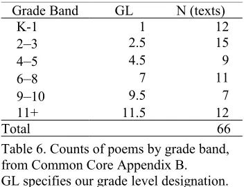
2010). Just as other materials from that source, the poems are classified into grade bands, as estab-lished by expert instructors. Table 6 provides the breakdown by grade band. Text length in this set ranges between 21 and 1100 words, the average is 182, total word count is 12,030.
Grade Band GL N (texts)
K-1 1 12
2–3 2.5 15
4–5 4.5 9
6–8 7 11
9–10 9.5 7
11+ ' 11.5 12
[image:6.612.346.522.145.280.2]Total 66
Table 6. Counts of poems by grade band, from Common Core Appendix B. GL specifies our grade level designation.
We computed lexical tightness for all 66 poems using the same procedure as for the two larger text collections. For computing correlations, texts from each grade band where assigned grade level as lis-ted in Table 6. For the poetry dataset, LT has rather low correlation with grade level, r=-0.271 (p<0.002). Text length correlation with GL is
r=0.218 (p<0.04). Correlation of LT and text length is r=-0.261 (p<0.02). Partial correlation of LT and GL, controlling for text length, is r=-0.227 and only almost significant (p=0.069). In this data-set, the correlation of Flesch-Kincaid index (FKGL) with GL is r=0.291 (p<0.003) and Flesch Reading Ease (FRE) has a stronger correlation,
r=-0.335 (p<0.003).
On examining some of the poems, we noted that the LT measure does not assign enough importance to recurrence of words within a text. For example, PNPMI(voice, voice) is 0.208, while the ceiling value is 1.0. We modify the LT measure in the fol-lowing way. Revised Association Score (RAS) for two words a and b:
=1.0 if a=b (token repetition)
RAS(a,b) =0.9 if of same lemmaa and b are inflectional variants
= PNPMI(a,b) otherwise
For the set of 66 poems, LTR moderately correl-ates with grade level r=-0.353 (p<0.002). LTR cor-relates with text length r=0.28 (p<0.02). Partial correlation of LTR and GL, controlling for text length, is r=-0.312 (p<0.012). This suggests that the revised measure captures some aspect of com-plexity of the poems.
We re-estimated the regression model, using FRE readability and LTR, on all 1012 texts of set #1. We then applied this model for prediction of grade levels in the set of 66 poems. The model achieves a solid correlation with grade level, r=0.447 (p<0.0001).
3.5 Revisiting Prose
We revisit the analysis of our two main datasets, set #1 and #2, using the revised lexical tightness measure LTR. Table 7 presents correlations of grade level with LT and LTR measures. Evidently, in each case LTR achieves better correlations.
Subset N Correlation GL< Correlation GL<R Set #1
All 1012 -0.546 -0.605
Inf 429 -0.499 -0.561
Lit 488 -0.610 -0.659
Set #2 (Common Core)
All 168 -0.441 -0.492
Inf 54 -0.310 -0.336
Lit 56 -0.546 -0.662
Combined set
All 1180 -0.528 -0.587
Inf 483 -0.472 -0.531
[image:7.612.87.281.329.494.2]Lit 544 -0.601 -0.655
Table 7. Pearson correlations of grade level (GL) with lexical tightness (LT) and revised lexical tightness (LTR). All correlations are significant with p<0.04.
We re-estimated a linear regression model using the grade level as a dependent variable and Flesch-Kincaid score (FKGL) and LTR as the two inde-pendent variables. The results of regression model on 1012 texts of dataset #1, R2=0.583,
F(2,1009)=706.07, p<0.0001, indicate that the amount of explained variance in the grade levels, as measured by the adjusted R2 of the model,
im-proved from 0.497 (with FKGL alone, r=0.705) to 0.582 (FKGL with LTR, r=0.764), that is absolute improvement of 8.5%. For comparison, the regres-sion model with LT explained 0.564 of the vari-ance, with 6.7% improvement over FKGL alone.
We re-estimated separate regression models for informational and literary subsets of set #1. For in-formational texts, the model has R2=0.667,
F(2,426)=426.8, p<0.0001, R2 improving from
0.651 (with FKGL alone, r=0.807) to adjusted R2
0.666 (FKGL with LTR, r=0.817). Regression model with LT brought an improvement of 1.2%, the model with LTR provides 1.5%.
A regression model was estimated on the literary texts of dataset #1. The result (R2=0.560,
F(2,485)=308.5, p<0.0001) reveals that adjusted R2
of the model rose from .453 (with FKGL alone,
r=0.673) to 0.558 (FKGL with LT, r=0.748), that is 10.5% absolute improvement. For comparison, LT brought 6.3% improvement. As with the origin-al LT measure, LTR provides the bulk of improve-ment for evaluation of literary texts.
The regression model (FKGL with LTR), estimated on all 1012 texts of set #1, is tested on 168 texts of set #2. In set #2, FKGL alone correlates with grade level with r=0.487, and the prediction formula achieves correlation of r=0.585 (the difference between correlation coefficients is statistically significant, p<0.001). The amount of explained variance rises from 23.7% to 34.3%, that is 10.6% absolute improvement. Even better result of predicting grade level in set #2 is achieved using a regression model of Flesch Readability Ease (FRE) and LTR, estimated on all 1012 texts of set #1. This model achieves correlation of r=0.616 (p<0.0001) on the 168 texts of set #2, explaining 37.9% of the variance.
For complexity estimation, in both proze and poetry, LTR is more effective than simple LT.
4 Related Work
Traditional readability formulae use a small num-ber of surface features, such as the average sen-tence length (a proxy for syntactic complexity) and the average word length in syllables or characters (a proxy to vocabulary difficulty). Such features are considered linguistically shallow, but they are surprisingly effective and are still widely used (DuBay, 2004; Štajner et al., 2012). The formulae or their features are incorporated in modern read-ability classification systems (Vajjala and Meurers, 2012; Sheehan et al., 2010; Petersen and Osten-dorf, 2009).
various manifestations of text-related readability. Peterson and Ostendorf (2009) compute a variety of features: vocabulary/lexical (including the clas-sic 'syllables per word'), parse features, including average parse-tree height, noun-phrase count, verb-phrase count and average count of subordinated clauses. They use machine learning to train classi-fiers for direct prediction of grade level. Vajjala and Meurers (2012) also use machine learning, with a wide variety of features, including classic features, parse features, and features motivated from studies on second language acquisition, such as Lexical Density and Type-Token Ratio. Word frequency and its derivations, such as proportion of rare words, are utilized in many models of com-plexity (Graesser et al., 2011; Sheehan et al, 2010; Stenner et al., 2006; Collins-Thompson and Callan, 2004).
Inspired by psycholinguistic research, two sys-tems have explicitly set to measure textual cohe-sion for estimations of readability and complexity: Coh-Metrix (Graesser et al., 2011) and Sour-ceRater (Sheehan et al., 2010). One notion of cohe-sion involved in those two systems is lexical cohe-sion – the amount of lexically/semantically related words in a text. Some amount of local lexical cohe-sion can be measured via stem overlap of adjacent sentences, with averaging of such metric per text (McNamara et al., 2010). However, Sheehan et al. (submitted) demonstrated that such measure is not well correlated with grade levels.
Perhaps closest to our present study is work re-ported in Foltz et al. (1998) and McNamara et al. (2010). These studies used Latent Semantic Ana-lysis, which reflects second order co-occurrence associative relations, to characterize levels of lex-ical similarity for pairs of adjacent sentences with-in paragraphs, and for all possible pairs of sen-tences within paragraphs. McNamara et al. have shown success in distinguishing lower and higher cohesion versions of the same text, but have not shown whether that approach systematically ap-plies for different texts and across grade levels.
Our study is a first demonstration that a measure of lexical cohesion based on word-associations, and computed globally for the whole text, is an in-dicative feature that varies systematically across grade levels.
In the theoretical tradition, our work is closest in spirit to Michael Hoey’s theory of lexical priming (Hoey, 2005, 1991), positing that users of language
internalize patterns of word co-occurrence and use them in reading, as well as when creating their own texts. We suggest that such patterns become richer with age and education, beginning with the most tight patterns at early age.
5 Conclusions
In this paper we defined a novel computational measure, lexical tightness. It represents the degree to which a text tends to use words that are highly inter-associated in the language. We interpret lexical tightness as a measure of intra-text global cohesion.
This study presented the relationship between lexical tightness and text complexity, using two datasets of reading materials (1180 texts in total), with expert-assigned grade levels. Lexical tight-ness has a significant correlation with grade levels: about -0.6 overall. The correlation is negative: texts for lower grades are lexically tight, they use a higher proportion of mildly and strongly inter-associated words; texts for higher grades are less tight, they use a lesser amount of inter-associated words. The correlation of lexical tightness with grade level is stronger for texts of the literary genre (fiction and stories) than for text belonging to in-formational genre (expositional).
While lexical tightness is moderately correlated with readability indexes, it also captures some aspects of prose complexity that are not covered by classic readability indexes, especially for literary texts. Regression analyses on a training set have shown that lexical tightness adds between 6.7% and 8.5% of explained grade level variance on top of the best readability formula. The utility of lexical tightness was confirmed by testing the regression formula on a held out set of texts.
Lexical tightness is also moderately correlated with grade level (-0.353) in a small set of poems. In the same set, Flesch Reading Ease readability formula correlates with grade level at -0.335. A regression model using that formula and lexical tightness achieves correlation of 0.447 with grade level. Thus we have shown that lexical tightness has good potential for analysis of poetry.
References
Baroni M. and Lenci A. 2010. Distributional Memory: A General Framework for Corpus-Based Semantics.
Computational Linguistics, 36(4):673-721.
Beigman-Klebanov B. and Flor M. 2013. Word Association Profiles and their Use for Automated Scoring of Essays. To appear in Proceedings of the 51th Annual Meeting of the Association for Computational Linguistics, ACL 2013.
Bouma G. 2009. Normalized (Pointwise) Mutual Information in Collocation Extraction. In: Chiarcos, Eckart de Castilho & Stede (eds), From Form to Meaning: Processing Texts Automatically, Proceedings of the Biennial GSCL Conference 2009, 31–40, Gunter Narr Verlag: Tübingen.
Brants T. and Franz A. 2006. “Web 1T 5-gram Version 1”. LDC2006T13. Linguistic Data Consortium, Philadelphia, PA.
Bullinaria J. and Levy J. 2007. Extracting semantic representations from word co-occurrence statistics: A computational study. Behavior Research Methods, 39:510–526.
Church K. and Hanks P. 1990. Word association norms, mutual information and lexicography. Computational Linguistics, 16(1):22–29.
Coleman, M. and Liau, T. L. 1975. A computer readability formula designed for machine scoring.
Journal of Applied Psychology, 60:283-284.
Collins-Thompson K. and Callan J. 2004. A language modeling approach to predicting reading difficulty.
Proceedings of HLT / NAACL 2004, Boston, USA. Common Core State Standards Initiative (CCSSI) 2010.
Common core state standards for English language arts & literacy in history/social studies, science and technical subjects. Washington, DC: CCSSO & National Governors Association.
http://www.corestandards.org/ELA-Literacy
DuBay W.H. 2004. The principles of readability. Impact Information: Costa Mesa, CA. http://www.impact-information.com/impactinfo/readability02.pdf Evert S. 2008. Corpora and collocations. In A. Lüdeling
and M. Kytö (eds.), Corpus Linguistics: An International Handbook, article 58. Mouton de Gruyter: Berlin.
Flesch R. 1948. A new readability yardstick. Journal of Applied Psychology, 32:221-233.
Flor M. 2013. A fast and flexible architecture for very large word n-gram datasets. Natural Language Engineering, 19(1):61-93.
Foltz P.W., Kintsch W., and Landauer T.K. 1998. The measurement of textual coherence with Latent Semantic Analysis. Discourse Processes, 25:285-307.
Fountas I. and Pinnell G.S. 2001. Guiding Readers and Writers, Grades 3–6. Heinemann, Portsmouth, NH.
Graesser, A.C., McNamara, D.S., and Kulikowich, J.M. Coh-Metrix: Providing Multilevel Analyses of Text Characteristics. Educational Researcher, 40(5): 223–234.
Graff, D. and Cieri, C. 2003. English Gigaword. LDC2003T05. Linguistic Data Consortium, Philadelphia, PA.
Gunning R. 1952. The technique of clear writing. McGraw-Hill: New York.
Heilman, M., Collins-Thompson, K., Callan, J. and Eskenazi, M. 2006. Classroom success of an intelligent tutoring system for lexical practice and reading comprehension. In Proceedings of the Ninth International Conference on Spoken Language Processing, Pittsburgh, PA.
Hiebert, E.H. 2011. Using multiple sources of information in establishing text complexity. Reading Research Report 11.03. TextProject Inc., Santa Cruz, CA.
Hoey M. 1991. Patterns of Lexis in Text. Oxford University Press.
Hoey M. 2005. Lexical Priming: A new theory of words and language. Routledge, London.
Kincaid J.P., Fishburne R.P. Jr, Rogers R.L., and Chissom B.S. 1975. Derivation of new readability formulas for Navy enlisted personnel. Research Branch Report 8-75, Millington, TN: Naval Technical Training, U.S. Naval Air Station, Memphis, TN.
Manning, C. and Schütze H. 1999. Foundations of Statistical Natural Language Processing. MIT Press, Cambridge, MA.
McNamara, D.S., Louwerse, M.M., McCarthy, P.M. and Graesser A.C. 2010. Coh-metrix: Capturing linguistic features of cohesion. Discourse Processes, 47:292-330.
McNemar, Q. 1955. Psychological Statistics. New York, John Wiley & Sons.
Mitchell J. and Lapata M. 2008. Vector-based models of semantic composition. In Proceedings of the 46th Annual Meeting of the Association for Computational Linguistics, 236–244, Columbus, OH. Mohammad S. and Hirst G. 2006. Distributional
Measures of Concept-Distance: A Task-oriented Evaluation. In Proceedings of the 2006 Conference on Empirical Methods in Natural Language Processing (EMNLP 2006), 35–43.
Nelson J., Perfetti C., Liben D., and Liben M. 2012. Measures of Text Difficulty: Testing their Predictive Value for Grade Levels and Student Performance. Student Achievement Partners. Available from http://www.ccsso.org/Documents/2012/Measures %20ofText%20Difficulty_final.2012.pd f
Petersen S.E. and Ostendorf M. 2009. A machine learning approach to reading level assessment.
Computer Speech and Language, 23: 89–109.
Senter R.J. and Smith E.A. 1967. Automated Readability Index. Report AMRL-TR-6620. Wright-Patterson Air Force Base, USA.
Sheehan K.M., Kostin I., Napolitano D., and Flor M. TextEvaluator: Helping Teachers and Test Developers Select Texts for Use in Instruction and Assessment. Submitted to The Elementary School Journal (Special Issue: Text Complexity).
Sheehan K.M., Kostin I., Futagi Y., and Flor M. 2010. Generating automated text complexity classifications that are aligned with targeted text complexity standards. (ETS RR-10-28). ETS, Princeton, NJ. Sheehan K.M., Kostin I., and Futagi Y. 2008. When do
standard approaches for measuring vocabulary difficulty, syntactic complexity and referential cohesion yield biased estimates of text difficulty? In B.C. Love, K. McRae, & V.M. Sloutsky (eds.),
Proceedings of the 30th Annual Conference of the Cognitive Science Society, Washington DC.
Sheehan K.M., Kostin I., and Futagi Y. 2007. SourceFinder: A construct-driven approach for locating appropriately targeted reading comprehension source texts. In Proceedings of the 2007 workshop of the International Speech Communication Association, Special Interest Group on Speech and Language Technology in Education, Farmington, PA.
Štajner S., Evans R., Orăsan C., and Mitkov R. 2012. What Can Readability Measures Really Tell Us About Text Complexity? In proceedings of workshop on Natural Language Processing for Improving Textual Accessibility (NLP4ITA 2012), 14-22. Stenner A.J., Burdick H., Sanford E., and Burdick D.
2006. How accurate are Lexile text measures?
Journal of Applied Measurement, 7(3):307-322. Turney P.D. 2001. Mining the Web for Synonyms:
PMI-IR versus LSA on TOEFL. In proceedings of
European Conference on Machine Learning, 491– 502, Freiburg, Germany.
Turney P.D. and Pantel P. 2010. From Frequency to Meaning: Vector Space Models of Semantics.
Journal of Artificial Intelligence Research, 37:141-188.
Vajjala S. and Meurers D. 2012. On Improving the Accuracy of Readability Classification using Insights from Second Language Acquisition. In proceedings of The 7th Workshop on the Innovative Use of NLP for Building Educational Applications, (BEA-7), 163–173, ACL.
Zhang Z., Gentile A.L., Ciravegna F. 2012. Recent advances in methods of lexical semantic relatedness – a survey. Natural Language Engineering, DOI: http://dx.doi.org/10.1017/S1351324912000125
Appendix A
The list of stopwords utilized in this study:
a, an, the, at, as, by, for, from, in, on, of, off, up, to, out, over, if, then, than, with, have, had, has, can, could, do, did, does, be, am, are, is, was, were, would, will, it, this, that, no, not, yes, but, all, and, or, any, so, every, we, us, you, also, s