Reliability assessment from fatigue micro crack data

IEEE TRANSACTIONS ON RELIABILITY, VOL. 46, NO. 2, 1997 JUNE 165

Reliability Assessment froim Fatigue Micro-Crack Data

Simon

P.

Wilson

David Taylor

Trinity

College, Dublin

Trinity College, Dublin

Key Words

-

Bayes inference, Coalescence, Fatigue, Gibb’tr sampling, Hierarchical model, Kernel density estimate, Micro- crack, Propagation

Summary & Conclusions - Micro-cracks are generally defmetl to be cracks less than 1 mm in length, which propagate under cyclic: stresses until they grow large and cause failure in an item (eg, corn,. ponent or structure). This paper proposes a method of using data on ‘fatigue micro-crack growth in a material’ to predict its reliabili-

ty. It is increasingly important to model such cracks effectively. Their growth properties, which differ in several respects from larger cracks, are discussed.

The paper develops a hierarchical model for the propagation of micro-cracks in a material. This stochastic model attempts to model the dependence of growth on local conditions, varying throughout the material, that causes variation in growth rates across the specimen. Given the model, data on micro-crack growth are used to compute posterior distributions of model parameters, from which a predictive distribution for reliability can be calculated. Computation of the posterior distributions is by Gibb’s sampling: and kernel density estimation. The methodology is illustrated with two data sets, one simulated and the other from a cast-iron specimen. Some possibilities for further work are presented.

1. INTRODUCTION & OVERVIEW

ACrOny”

MCMC Monte Carlo Markov chain.

When a metal item (eg, structure or component) is subject to a cyclic load, it generally fails eventually2. Thus it is im- portant - from a safety, legal, financial, and academic perspec tive - to predict when this fatigue failure is likely to occur. Fatigue failure of a metallic item occurs because cracks pro- pagate through it, and this propagation is a function of several internal & external factors: eg, size of load, microstructural pro- perties of the material, temperature, humidity.

Broadly speaking, crack propagation has 5 phases. 1. Dormant. There are no cracks in the material.

2. Nucleation. The crack is initially formed.

3. Micro-crack growth. The crack grows rather haphazard-. ly up to about 1 mm in length.

’The singular & plural of an acronym are always spelled the same. ’Some ferrous materials appear to have a fatigue limit, below which the item does not fail.

4. Macro-crack growth. The crack continues to propagate before its growth rate finally increases dramatically.

5 . Failure. The component fails; this occurs very quickly, relative to the other phases, and can be ignored as a factor in

determining reliability. 4

Out of the many cracks that nucleate and become micro- cracks in a specimen, usually there is only one that becomes dominant and causes failure. The fact that only one macro-crack is important makes the modeling of phase #4 rather easier than the others. There are many situations in which the macro-crack phase #4 is the longest phase in the specimen life. Thus, most of the considerable body of work on crack propagation is devoted to macro-cracks.

Nevertheless, the micro-crack phase can form a very sizeable proportion of the failure time - 60 % is typical for some

materials - particularly in situations of relatively low stress levels where lifetimes are long. Figure 1 [ 11 shows this for two specimens of a molybdenum steel. Such situations are very com- mon where, for example, components have been designed to withstand stresses considerably above those that they actually encounter. Because the reliability of many components is im- proving, micro-crack behavior is becoming a critical factor in determining reliability, So in terms of quantifying component lifetime and as a factor to be considered in the design process, models for the micro-crack phase are increasingly important. Once a crack has attained a certain threshold size, failure occurs very rapidly. So, to determine component reliability, a model for crack propagation is proposed and used to calculate when the length of the largest crack exceeds the threshold.

0 2.5 50

75

100

Percentsage of lifetime

I

1: No cracks present

2: Nucleation

3 : Micro-crack

4/5:

Macro-crack Xr;

[image:1.599.301.541.491.591.2]

i

failure

Figure 1. Time Spent in Phases of Crack Growth [for two specimens of molybdenum alloy]

Three properties of micro-cracks make macro-crack models inappropriate:

1. The usual models for macro-cracks cannot accommodate the various features of micro-crack growth. Section 2 proposes a modification of the usual macro-crack model that accounts for these differences.

166 IEEE TRANSACTIONS ON RELIABILITY, VOL. 46, NO. 2. 1997 JUNE

3. Micro-crack growth is a function of varying local con-

ditions in the material. 4

Section 3 argues that a stochastic hierarchical model is a good first step in modeling the randomness & s-dependencies between the collection of micro-cracks. Section 4 describes how statistical inference and reliability prediction can be conducted using MCMC, and provides two illustrations using data on micro-crack growth.

Notation

a , a ( t ) crack length at time t AK stress intensity range C, n , Q

ACT stress range a0 initial crack length

d diameter of a grain in the material microstructure

D distance from the point of crack nucleation to where the crack encounters the first grain boundary

N number of micro-cracks in a specimen

f ( a , d ; 0) empirical function of a , d , and parameter 0

m, q5 grain boundary specific constants, 0 5 $ 5 1 I index for cracks; i= 1,2,. . . ,N unless otherwise

specified

.i

index for times; j = 1,2,. . . ,k unless otherwise specified

mi, q5i [ m ,

41

for crack i

aij _{observed crack length for crack} i at t i m e j A , ( t ) length of crack i at time t , a r.v.

A { a . 11’ ,. i = 1 , ..., N ; j = l ,

...

k } .

Other, standard notation is given in “Information for Readers

& Authors” at the rear of each issue.

material specific constants

logit(q5i) log(+;) - log(l-4i)

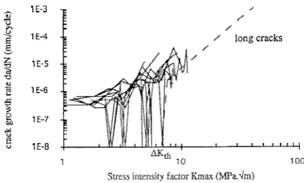
can be smooth but can involve periods of stationarity and the possibility of being stopped altogether. This can be observed by plotting crack-growth vs crack-length for a set of cracks in a metal; figure 2 [ 3 ] is a typical plot. This widely observed phenomenon is caused by the crack encountering a boundary between grains in the material microstructure; at such a boun- dary, growth rate is slowed by a factor that depends on local conditions. In this way, some micro-cracks propagate to become macro-cracks with hardly any delay while others are held back for some time or even stopped altogether. The difference in the length at which cracks slow down is due to the different distance that the cracks progress before hitting a grain boundary.

-

?-

E

,

/

/

3

1E-4 / long cracks

E v

1E-5

s

5

5 1E-6

&, 1E-7

1E-8 6

1 0

[image:2.599.324.545.231.364.2]

Stress intensity factor h a x (Wa.dmim) Figure 2. Typical Growth Behavior of Micro-Cracks

The general approach to modeling the effect of a grain boundary is to take the Paris-Erdogan equation and multiply

the r.h.s by a factor that accounts for the local conditions at the first grain boundary:

da

2. MICRO-CRACK PROPAGATION: WORK TO DATE dt

~ = C - ( A K ) n - f ( a , d ;

e),

(3)

Thef( a,d; 19) is usually increasing in the distance from the first grain boundary. A variety of forms for

f

have been proposed that empirically capture this property; eg, Miller et al simply propose

[4]:

2.1 Previous Work

The usual model for large macro-crack growth is the Paris- Erdogan equation [2: chapter 11 which defines:

a ( 0 ) = ao.

where, usually,

(1)

( 2 )

f = a - d , for a

<

d ,

while Plumtree & Schafer suggest [ 5 ] :

f = 1 - 4 - ( ( d - a ) / d ) ’ , for a constant 4.

However, there is no consensus on the best form forf: it ap- pears to vary for different materials.

To solve (1) uniquely, a. is needed. This model has been used successfully to describe the observed propagation of a domi- nant macro-crack in many experiments and the values of C & n have been established for a wide range of materials.

The growth of a macro-crack is as smooth as the use of such a differential equation model implies. This is in stark con- trast to what we observe for micro-cracks, whose progression

2.2 Micro-Crack Model with an Exponential Local Term

One model of the form in (3) is:

= C. (AK)’-[1 - +-exp(-m. ( u - D ) ~ ) ] , (4)

WILSON/TAYLOR: RELIABILITY ASSESSMENT FROM FATIGUE MICRO-CRACK DATA

D is a function of d.

Eq

(4)

& ( 5 ) for da/dt is the Paris-Erdogan rule multiplied by the local factor:

The size of the slowdown in growth at the grain boundary is governed by 6:

If

4

= O then there is no local effect and the crack moves ac-

If

4

= 1 then when U = D (when the crack hits the first grain cording to Paris-Erdogan.

boundary), d u ( t ) / d t = O and the crack is stopped.

The m is a scaling factor that controls how far away from the boundary the local effect is important:

If m is small, then the crack slows down a long distance from

If m is large, then the crack slows down a short distance from the boundary.

the boundary.

The use of an exponential measure of distance forf(a, d ; 6) is new. The advantage of such a measure is that it is increas- ing but bounded in the distance from

D.

Thus, as

a

progresses beyond D, the exp(--m- ( a -

D )

2 , becomes smaller and

du ( t ) /dt becomes closer & closer to the usual Paris-Erdogan equation for macro-cracks. However it remains empirical and, like all proposed forms forf, has not been derived by consider- ing more fundamental processes of crack growth.

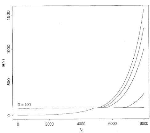
A solution for a(t) is not available in closed form but can be efficiently obtained with a second order finite difference ap- proximation. The solution is shown in figure 3 for:

5 values of

4

= 0.6 (the fastest growing), 0.7, 0.8, 0.9, 1

C = 0.2, Au = 10, n = 1, m = 0.02, Q = 1, D = 80. The crack growth does indeed slow around the value of D, with the extent of the slowdown, depending on the size of

4.

(the slowest growing)

3 . EXTENDING TO A RANDOM MODEL

FOR MANY MICRO-CRACKS

There has been some work on random models for micro-. crack propagation, although the work is small compared withi that for macro-cracks. Cox & Morris define a model through1 a growth-control parameter that evolves as a Markov chain [ 6 ] . Taylor has introduced the concept of a P-a plot to describe the: probability of growth of a crack in a given number cycles as

a function of crack length [7]. Our approach treats the

parameters of the deterministic model as r.v. This concept has been used for macro-crack models, such as the work of Paluszny

& Nicholls on a model for crack growth in ceramics [8]. Tcr

our knowledge, the idea has not been applied to micro-crack. models.

I /

0 2000 4000 6000 8000

N

[image:3.601.302.545.62.278.2]

Solutioin for a ( t ) vs

+

Figure 3.

3.1 General

We have established a deterministic model for a single micro-crack in terms of parameters: C, n, m,

4,

. . . . Stage #2

of the modeling process is to extend the model to many cracks, growing broadly in the same manner but with variations accor- ding to local conditions. A simple tractable form for such a col- lection of similar entities is a hierarchical model, which describes the cracks as a set of random, exchangeable objects, conditionally s-indlependent of each other, given local condi- tions around each crack.

Assumptions

1. N is a constant for a given specimen. 2. n, C, ACT, are known.

3 . The local conditions at each crack are described by the

4. Conditional on the local parameters, a. each crack is s-independent.

b. the deterministic model of (5) gives a solution for a, ( t ) .

5. A, ( t ) has a Gaussian distribution with mean a, ( t ) and standard deviation a-a, ( t ) .

6. The use of multiplicative error for A, ( t ) is necessary because crack lengths vary over several orders of magnitude with time.

7a. The local parameters are r.v. that come from some underlying common probability distribution.

7b. The log ( m , ) are s-independent and have a Gaussian distribution with mean M and standard deviation a,.

7c. The logit($,) have a Gaussian distribution with mean

$ and standard deviation u4.

8. Statistical inference is Bayes3. Thus prior degrees-of-

4

local parameters m,,

Di,

4,.

belief on

M ,

a i

+,

u i , d, a2 are required.

168 IEEE TRANSACTIONS O N RELIABILITY. VOL. 46, NO. 2, 1997 JUNE

The distribution of the D, can be obtained from geometrical considerations and is a function of grain diameter

d The evaluation of this distribution is addressed in section 3 2.

This hierarchical model is often visualized as a directed graph

their influences on each other. Each node represents one part

100000

Samples

(D

0

0 0

which represents all the quantities of interest in the model and

of the model and is s-independent of all other nodes in the graph, conditional on its parents (the nodes that point directly to it).

*

> O -

$ O~

(n

c m

a

0 A solid line between nodes indicates a random relationship

between nodes (the parent is a parameter in the distribution

r

of the child). 0

between the two connected nodes.

* A dotted line indicates a logical or deterministic relationship

A box around nodes indicates a set of variables that are con-

0

0

0 0 0 5 1 0 15 20

D

ditionally s-independent given their parents, 4

[image:4.605.312.527.74.299.2] [image:4.605.59.273.293.473.2]

Figure 5. Simulated Density of D [d= 1 , circular grains] Figure 4 is the directed graph that represents this model.

Figure 4. Directed-Graph Representation of the Hierarchical Model

The strengths of the hierarchical model are not only in its tractability. The cracks are unconditionally s-dependent, but the similarity between each crack is maintained since the marginal distribution of

A i

( t ) is the same for all i (a result of assump- tions #4a, #5, #7a).

3 . 2 Prior Distribution for D

D

= --R.cos(O

-

$)

+

[ % d 2

-

R2.sin2(8-$)]”, ( 6 ) In the absence of more specific information for this exam- ple, assume that R, 19. $ are uniformly distributed r.v. over their possible values, then one can generate values from the distribu- tion of D by direct simulation. Figure 5 is a histogram of the 4 More generally, d itself varies; indeed, the distribution of grain diameters is easily observed and has been quantified for many materials. This generalization presents no problem to the direct simulation of the distribution of

D.

Other, perhaps more realistic, geometries for the grains could be used, e g , Voronoi tessellations. Direct simulation of a distribution for D is available, although more complex. The problem can be considered in all 3 dimensions, and used with spheres or 3-dimensional Voronoi tessellations, However, since crack growth often occurs in one direction, perpendicular to the stress axis, a 2-dimensional geometry is usually sufficient. We are interested only in a prior distribution for D that is up- dated, given our data on crack growth, the use of the simpler prior from an assumption of circular grains might be all that is needed.

resulting values of D when d is fixed at 1.

4. STATISTICAL INFERENCE AND RELIABILITY ASSESSMENT

A very simple example shows how we find our prior

Assumptions degree-of-belief.

Examp le

9. We have data on N cracks. The length of each crack is observed at times tl,t2, ..., tk

There are 2 dimensions, and the grains are circular with

tion ( R , 0) in polar co-ordinates. It then proceeds at an angle $ (clockwise from the positive x-axis) until it hits the boundary of the circle. The length of the line from nucleation point to circle perimeter is D . Thus (by the cosine rule):

10. To simplify, ai,l = a. of the crack, as required to 4 a diameter d . A crack nucleates at a point in the circle at a posi- solve ( 5 ) .

*

WILSON/TAYEQR: RELIABILITY ASSESSMENT FROM FATIGUE MICRO-CRACK DATA

Given the data, the statistical analysis has 3 objectives: Estimate model parameters. Because we adopted Bayes in- ference, the goal is to obtain posterior distributions of the parameters, conditional on A .

Predict the progression of cracks in other specimens of the same material.

Predict the future propagation of the observed cracks. This is important because it can be used to predict the reliability,

4

To conduct s-inference with this model, obtaining posterioi- or time to failure, of the specimen.

distributions of parameters and predictive distributions, is a com- putational challenge. Recent advances in stochastic simulation techniques - in particular, MCMC

-

meet the challenge, s-inference is quite feasible using a machine of moderate com. putational power, eg, the results in section 4.3 took a few hours on a Pentium PC.

4.1 Parameter Estimation

The model has many parameters: Each crack has 3 parameters - mi, Di,

&.

The global distributions of mi,

Di,

c$~ are described by

4

parameters M , 0; d,

a,

G,$ The multiplicative error 02.

Thus, for N cracks, there are 3N

+

6 parameters.

The parameters are partitioned in 2 groups: local andl global. On the local level, crack i is described by its 3 locall parameters; estimation of mi, Dj, &, U* yields specific infor-.

mation about the performance of each crack. On the global level, the distribution of the population of local parameters in the! specimen is estimated, ie, M , 0; d,

+,

0:.

MCMC for simple hierarchical models is usually perform- ed with the Gibb’s sampler, and we use it here [9: and its; references]. The sampler does not require one to be able to Sam-. ple from the posterior distribution of each parameter, but rather thehll conditionals for each parameter, or the distribution con-. ditional on the data and all other parameters. The full condi-. tional for any parameter can be obtained by looking at the joint distribution of data and parameters as a function of the parameter in question; in this paper, combining all the distributional and s-independence assumptions in section 3 (viz, assumptions #1,

#2, #4, # 5 , #7b, #7c, #8

-

#lo), this joint distribution is:

i = l ,

...,

N , j = l ,

...,

k; U’, M , U; d, @, U;)

1

(7)

a, ( t J ) = solution to the model ( 5 ) with m,, D,, 9,, and a. =

a form for f(

D,

Id) is explained in section 3.1

-.() denotes the prior distributions on hyper-parameters. %19

A sample from each full conditional distribution is calculated differently. For the full conditionals of m,, D,,

4,,

calculation of the pdf requires that a,

($1,

for i = 1,.

.

.

,k, be computed; this is a slow process. Thus, for these parameters, the griddy Gibb’s sampler is used [lo], evaluating the full con- ditional at 5 points. For the hyper-parameters, the pdf‘s are of

a form that is easy to evaluate, and a sampling is done from a discrete approximation to the continuous distribution.

The output from the sampler is a set of values of each parameter that are random samples from the relevant posterior distribution. These: values can be used to estimate the posterior distribution, either by combining them into a histogram or by using one of the kernel density estimation techniques [9, 111, Predictive pdf‘s for future values of crack length can be ob- tained in a similar manner.

4.2 Predicting Reliability Notation

Ath a given threshold size

T life-length of specimen

G )

L

implies: sample j , j = 1,2,. . . ,L

number of samples produced by Gibb’s sampler from posterior distributions of the local parameters.

Assumption

11. Specimen reliability is estimated by predicting the time at which the first crack reaches A,, conditional on A .

Pr{T

>

t l A } = l’r{maxi{Ai(t)}

s

AhIA}

The conditional s-independence of the Ai are used to estimate the joint posterior distribution of all the crack lengths at any time t with the kernel estimate:

170 IEEE TRANSACTIONS ON RELIABILITY. VOL. 46. NO. 2, 1997 JUNE

ai(t) is the solution to (5) with parameters mp), D p ) ,

+i(i).

Use this approximation in (8); the reliability is:

4.3 Application to Data

Two sets of data are analyzed. In both cases, vague prior distributions were placed on the hyper-parameters:

a Gaussian distribution with mean 0 and standard deviation

1000 on M and

a,

inverse Gamma distributions with ‘scale parameter = 0.5’

and ‘shape parameter = 0.5’ for a’, ~7: and 0;. For the prior

distribution of D , we assumed little prior information available on the grain diameters d, except that an upper bound to d was 500; thus (6) was used to form the prior distribution on each

D i

from a uniform distribution on [0, 2x1; where 0, J / , R were chosen uniformly on [0,500].

4.3.1 Data Set #1

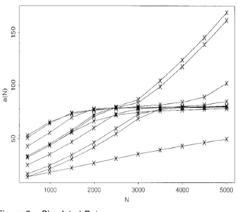
This is a simulated set of lengths from N = 10 cracks, taken

from a solution to ( 5 ) . The crack lengths were observed at k = 10 time points. Figure 6 shows the 10 cracks with the observed-lengths marked.

0

in

r

0

0

h r

z

m

1

0

1000 2000 3000 4000 5000

N

Figure 6. Simulated Data

The data were analyzed using the Gibb’s sampler; lo3

samples from all the posterior distributions were generated. The first 300 were ignored and the results calculated using the re- maining 700 samples. With N = 10, there are 36 parameters to be estimated from 100 data points, so that the posterior distribu- tions for the crack specific parameters m, D , q5 were not very informative. Figure 7 shows the kernel pdf estimates of the

posterior distributions of the mean & variance of log@) and logit(q5). Figure 8 shows the estimate of the future reliability, with &=1000, of the specimen to be fairly precise, with failure predicted to occur “almost certainly” between t= 14 and

t= 16.

Figure 7 . Kernel Posterior pdf Estimates for 4 Global Parameters

[given the data from the simulated specimen with 10 micro-cracks]

m

0

W

P O

-1

5

n

a b

0

N

0

0

0

12000 13000 14000 15000 16000 17000 18000 N

Figure 8. Estimated Reliability of Simulated Specimen

[with: 10 micro-cracks, At,,= 10001

4.3.2 Data Set #2

[image:6.601.316.552.156.373.2] [image:6.601.312.557.427.653.2] [image:6.601.49.293.428.646.2]

WILSONiTAYLOR: RELIABILITY ASSESSMENT FROM FATIGUE MICRO-CRACK DATA

[image:7.600.42.287.177.643.2] [image:7.600.45.286.185.399.2]

the growth of cracks measured with the aid of a microscope. Figure 9 shows the observed lengths of 190 micro-cracks in the specimen. The lengths were observed at only 4 points; thurs our model is over-parameterized as regards estimation of in- dividual crack properties (since there are 3 parameters per crack). So we concentrate on the 6 global parameters and the reliability prediction. Figure 10 shows the predicted reliabili- ty, with Ath= 1000.

0

0

m

- 0

z::

0

?

1500 2000 2500 3000 3500 4000

N (~1000)

[from a cast-iron specimen]

Figure 9. Micro-Crack Data

--_\

\

\ \

8000 10000 12000 14000 16000

N (xl000)

Figure 10. Estimated Reliability of Cast-Iron Specimen

[with: At,,= lOOO]

Figure 9 shows that there is one dominant crack that is larger than the others; thus, in contrast to the simulated data, the reliability prediction is almost entirely dependent on the predicted growth of this crack alone.

5 . CLOSING REMARKS

One important aspect of micro-crack growth has been ig- nored in this approach: there is often a large spatial-dependence between micro-cracks. For example, neighboring cracks can coalesce, and the presence of a large crack can inhibit growth of cracks nearby. In some materials the main cause of growth in the micro-crack phase is coalescence. Coalescence occurred in some of the cracks of data set #2, and was resolved by con- sidering all the cracks that subsequently coalesced as one crack with length the sum of its constituents. This rather crude ap- proach can be improved upon, and presents an interesting modeling problem.

A practical reason for not incorporating a spatial compo- nent into the model, apart from the prospect of computational problems, is that dhe data on micro-crack growth does not pro- vide any information on the location of each crack in the specimen. This reflects the difficulty of 1) observing such small objects, and 2) accurately measuring them on a specimen. Even locating the same crack that was measured previously can be a problem. However, improvements in experimental techniques mean that spatial data ought to become possible to collect, at which point a spatial model approach can be pursued.

REFERENCES

A. Fathulla, B. Weiss, R. Stickler, “Short fatigue cracks in technical pm-Mo alloys”, [12: pp 115-1321

K. Sobczyk, B.F. Spencer, Random Fatigue: From Data to Theory, 1992; Academic Press.

V. Gros, C. Prioul, P. Bompard, “Initiation of short fatigue cracks in railway lines”, Fatigue ‘96: Proc. Sixth Int? Fatigue Congress (G.

Lutering, H. Nowack, E&), vol 1, 1996, pp 313-318; Pergamon. K.J. Miller, H.J. Mohamed, W.R. de 10s Rios, “Fatigue damage ac- cumulation above and below the fatigue limit”, [12: pp 491-5111,

A. Plumtree, S. Schafer, “Initiation and short crack behavior in aluminium alloy castings”, [12: pp 215-2271,

B.N. Cox, W.L. Morris, “A probabilistic model of short fatigue crack growth”, Fatigue & Fracture of Engineering Materials & Structures,

D. Taylor, “Short fatigue crack growth in cast iron described using P-a curves”, Int? J. Fatigue, vol 17, 1995, pp 201-206.

A. Paluszny, P. F. Nicholls, “Predicting time-dependent reliability of ceramic motors”, Ceramics for High Pefortnance Applications - I1 (J.J.

Burke, E.N. Leioe, R.N. Katz, E h ) , 1978, pp 95-112; Brook Hill. A.F.M. Smith, G.O. Roberts, “Bayesian computation via the Gibb’s sampler and related Markov chain Monte Carlo methods”, J. Royal Statistical Soc. 19, vol 55, 1993, pp 3-23.

M. A. Tanner, Tools for Statistical Inference: Methods for the Explora- tion of Posterior Distributions and Likelihood Functions, 1993; Springer-Verlag

.

A.E. Gelfand, A.F.M. Smith, “Sampling based approaches to calculating marginal densities”, J. Amer. Statisticalhsoc, vol85, 1990, pp 398-409.

The Behavior of Short Fatigue Cracks (K.J. Miller, E.R. de 10s Rios, V O ~ 10, 1987, pp 419-428.

E&), 1986: Mechanical Engineering Publishers.

AUTHORS

172 IEEE TRANSACTIONS ON RELIABILITY, VOL. 46, NO. 2, 1997 JUNE

Internet (e-mail): [email protected]

Simon Wilson is a lecturer in the Statistics Department of the Universi- ty of Dublin, Trinity College. He received his PhD in stochastic modeling from the George Washington University in Washington DC. His research interests lie in the application of Bayes statistics to engineering problems, such as fatigue crack growth, image processing, and software reliability.

Prof. David Taylor; Dep’t of Mechanical & Manufacturing Engineering; Trinity College; Dublin 2, Rep. of IRELAND.

David Taylor i s a professor in the Mechanical & Manufacturing Engineer- ing Department of the University of Dublin, Trinity College. He received his

PhD in materials science from Cambridge University. He has worked exten- sively in crack propagation in materials - publishing 3 books and about 70 papers on the subject. This work has concentrated on the application of frac- ture mechanics theory and its extensions into areas such as very slow crack growth.

Manuscript TR96-123 received 1996 August 29; revised 1997 May 12 Responsible editor: J.A. Nachlas

Publisher Item Identifier S 00 18-9529(97)05725-4 4 T R F

MA NUSCRIP TS RECEIVED M A NUSCRIP TS RECEIVED MANUSCRIPTS RECEIVED MANUSCRIPTS RECEIVED

“Evaluation of average cost for imperfect-repair model” (J. Lim, D. Park, et

al.), Dr. Dong Ho Park, Professor * Dept. of Statistics Hallym Univ. * 1 Okchon Dong Chunchon 200-702, Kangwon Do Rep. of KOREA. (TR97-016)

“Egocentric voting algorithms” (M. Azadmanesh, et al.), Dr. Mohammad H. Azadmanesh * Ctr. Mgmt. of Information Technology * 308 CBA Bldg * Univ. of Nebraska * Omaha, Nebraska 68182-0459 USA. (TR97-017)

“Integrating routing & survivability in fault-tolerant computer-network design” (S. Pierre, et al.), Samuel Pierre * LICEF, Tele-University Univ. of Quebec

-

CP 670, Succ C * Montreal, Quebec H2L 4L5 * CANADA.

“Estimating the number of errors in a system: Efficiency of removal, recapture, seeded-error methods” (C. Lloyd, P. Yip, et al.), Dr. Christopher J. Lloyd * Dept. of Statistics

-

The University of Hong Kong * Pokfulam Road

HONG KONG. (TR97-019)

“Complexity of distributed-problem reliability computation” (M. Lin, D. Chen), Min-Sheng Lin * Dep’t of Information Mgmt. * Tamsui Oxford Univ. College

-

32. Chen-Li Rd, Tamsui * Taipei 25103 TAIWAN - R.O.C.. (TR97-020)

(TR97-018)

“Robust distributed genetic algorithm for reliable network-topology design”

(A. Kumar, et al.), Dr. Anup Kumar * Eng’g Math. and Computer Science Dep’t

-

Univ. of Louisville a Louisville, Kentucky 40292

-

USA. (TR97-028) “Redundancy allocation to maximize a lower percentile of the system time-to-failure distribution” (D. Coit, A. Smith), Dr. David W. Coit * Dept. of Industrial Eng’g Rutgers Univ.

-

POBox 909

-

Piscataway, New Jersey “Bayes prediction for the linear-regression model with student-t error distribution” (V. Ng), Dr. Vee-Ming Ng * Dep’t of Mathematics & Statistics

-

Murdoch Univ. * Murdoch, WA 6150 AUSTRALIA. (TR97-030) “Design constraints of fault-tolerant level-mode sequential logic” (M. Meulen), Meine J.P. van der Meulen * SIMTECH

.

Oostmasslaan 71 3063 AN Rotterdam The NETHERLANDS. (TR97-03 1)

“An implicit method for incorporating common-cause failures in system analysis” (J. Vaurio), Dr. J. K. Vaurio * Imatran Voima Oy Loviisa Power Station * PL 23 SF-07901 Loviisa

“Testing exponentiality of the residual life based on dynamic Kullback-Lieber information” (N. Ebrahimi), Dr. Nader B. Ebrahimi

Dept. of Mathematical Sciences Northern Illinois University

-

DeKalb, 08855-0909 * USA. (TR97-029)

FINLAND. (TR97-032)

Division of Statistics “New ways to improve the analysis of step-stress testing” (J. McLinn), James Illinois 601 15-2888

.

USA. (TR97-033)

A. McLinn Re1:Tech Group 10644 Ginseng Lane Hanover, Minnesota

“Mean residual life of continuous lifetime distributions” (L. Tang, et al.), Dr. Loon Ching Tang * Dept. of Industrial & System Eng’g

-

National Univ. of 55341 * USA. (TR97-021)

”A tabu-search approach for designing computer-network topologies with unreliable components” (S. Pierre, A. Elgibaoui), Samuel Pierre LICEF,

Singapore * I O Kent Ridge Crescent * Singapore 119260 Rep. of SINGA- PORE. (TR97-034)

Tele-University

-

Univ. of Quebec * CP 670, Succ C Montreal, Quebec H2L “A simple method for considering node failures in evaluating network reliability” (S. Wang, et al.), Dr. Sheng-De Wang * Dept. Electrical Eng’g; EE Bldg, Rm 441 National Taiwan Univ. * Taipei 106 TAIWAN - R.O.C.. “An algorithm for coherent-system reliability” (T. Luo, K. Trivedi), Tong Luo

-

GTE Labs, MS 40 * 40 Sylvan Rd Waltham, Massachusetts 02254 USA. (TR97-024)

4L5 * CANADA. (TR97-022)

(TR97-023)

“Modeling the failure rate for Fokker F-27 tires using a neural network’’ (A AI-Garni, et al.), Dr. Ahmed 2. AI-Garni * Mechanical Eng’g Dept * King

Fahd Univ. of Petroleum & Minerals * Box 842 * Dhahran 3 1261 Kgdm. of SAUDI ARABIA, (TR97-035)

“Exponentiated exponential family: An. alternative to Gamma & Weibull distributions” (R. Gupta, et ai.), Rameshwar D. Gupta * Dept. Mathematics, Statistics, Computer Sci.

-

University of New Brunswick * POBox 5050

-

Saint John, New Brunswick E2L 4L5 CANADA. (TR97-037)

“Predicting reliability of a telecommunication system using a reliability Petri net” (S. Hong, et al.), Sung-Back Hong * ISDN Call Proc. Sec., ETRI

-

161 Kajong-Dong, Yusong-Gu * Taejon 305-350 Rep. of KOREA. (TR97-038) “Limited failure-data represented by a correction factor” (A. Gera), Dr. Amos

E. Gera Design QA Dept, 3495 * ELTA Electronics Industry Ltd

-

POBox 330 * Ashod 77102 * ISRAEL. (TR97-025)

“Reliability of mechanical components: Accelerated testing and statistical 58 rue J. Parot. St.

Etienne 42000 FRANCE. (TR97-026)

“Using statistics of the extremes for software-reliability analysis” (L. Kaufman, D. Smith, J. Dugan, B. Johnson), Dr. Joanne Bechta Dugan Dept. of Electrical Engineering * Thornton Hall University ofVirginia Charlottes- ville, Virginia 22903-2442 * USA. (TR97-027)

“Estimation O f the distribution of the life of complex systems, using SimukItiOn ofelement-lives” (J. Sanz-Juan, et al.), Dr. Jose Sanz-Juan Dept de Estadistica e 1.0.

-

Univ. Politecnica de Valencia * Camino de Vera s/n *

Valencia 46022

-

SPAM. (TR97-039)

“ A theory of independent fuzzy probabilities for reliability” (J. Dunyak, et al.), Dr. James Dunyak * Mathematics Dep’t

-

Texas Tech Univ. Box 3 1042