Zone Re
\
ning
C.-D. Ho and H.-M. Yeh, Tamkang University,
Taipei, Taiwan, ROC
Copyright^ 2000 Academic Press
Introduction
Zone reRning is a powerful tool for applying coupled melting and freezing operations for manipulating im-purities in crystals, as well as for separating liquid or solid mixtures. It wasRrst used to purify germanium in 1952. Zone reRning combines the well-known fact that a freezing crystal differs in composition from its corresponding liquid phase, so that passing a short heater along a solid ingot leads to a puriRcation of the ingot. For improving the separation efRciency and reducing time, a series of narrow heaters moving slowly over a solid ingot can be used in multi-pass zone reRning.
Several mathematical models have been presented for modelling multi-pass zone reRning processes when zone length affects the separation efRciency. Furthermore, variable cross-sectional area ingots with speciRed volumes have been introduced to im-prove the separation efRciency. Analogue simulators were used to simulate zone reRning by means of a single mathematical equation that expresses solute concentration as a function of distance for any initial distribution of solute and any number of passes through an ingot of a speciRed length. These simula-tors include liquid mechanical and electrical analogue simulators. Thousands of signiRcant papers devoted entirely or largely to some aspect of application of zone reRning have appeared in the last two decades. For instance, silicon-on-insulator (SOI) Rlms, and semiconducting and superconducting materials were prepared by zone reRning operations.
Separation Theory in Multi-pass
Operation
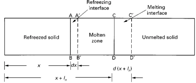
Eqn (1) can be derived by taking the mass balance within the moving zone ABCD or ABCD as
shown in Figure 1. It is based on the following as-sumptions: (a) constant distribution coefRcient; (b) uniform composition and no diffusion in the molten zone; (c) no change in density during melting and freezing; (d) a constant cross-sectional area for the ingot.
dCM n(Z)
dZ #
dYn(Z) dZ #k
Yn(Z)
CMn(Z)
"kCMn\1[Z#Yn(Z)] Yn(Z)
1#dYn(Z) dZ
,0)Z)1!Yn(Z) [1]
dCM n(Z)
dZ #
dYn(Z) dZ #k
Yn(Z)
CMn(Z)"0,
1!Yn(Z))Z)1 [2]
and the boundary conditions of eqns (1) and (2) become:
atZ"0, CMn" k Yn(0)
Yn(0)
0
CM n\1(Z) dZ [3]
atZ"1!Yn(Z),
CM n" k
Yn(Z)
1!1\Yn(Z)
0
CMn(Z) dZ
[4]in which:
CMn(Z)"Cn(x)/C0 [5]
Yn(Z)"ln(x)/L [6]
Figure 1 Schematic diagram of zone-refining operation.
The initial solute concentration of the ingot,C0, is uniform, the amount of solute,Wn,i, either transport-ing away from (k(1), or into (k'1) theith section after thenth pass, can be calculated by:
Wn,i"
xi#1
xi
#C0!Cn(x)#Adx [8]
Since the original amount of solute in the ingot is W0"ALC0, whereAis the cross-sectional area of the ingot, the fraction of solute removed,fn,i(Yn,i(Z)), in each section afternpasses, is expressed as:
fn,i(Yn,i(Z))" Wn,i
W0"
Zi#1
Zi
#1!CMn(Z)#dZ [9]
Once the values offn,i(Yn,i(Z)),i"1, 2,2,Ifor each section are known, the overall amount of solute re-moved Fn(Yn(Z)) can be obtained by summing up these values as:
Fn(Yn(Z))" I
i"l
fn,i"
M
i"l
fn,i"
1 2
M
i"l
fn,i [10]
wherexIis the place whereCn(x)"C0orCM n(Z)"1.
Normal Freezing
The optimal zone length Y*
1 for maximumFq(Y1) is obtained by solving the equation, dF1(Y1)/dY1"0, with the use of eqns (9) and (10), since dF1(Y1)/dY1is less than zero fork(1 and dF1(Y1)/dY1is larger than zero fork'1. In order to meet both requirements, therefore,Y1must be as large as possible, i.e. normal freezing for all values of the distribution coefRcient. Accordingly, the optimal zone length for the Rrst pass is:
l1"L or YH1"1 [11]
Varying Optimal Zone Length in Each Pass
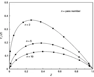
The optimal variable zone lengthYHn,i(Z), the corre-sponding concentration distribution CMHn(Z) and the fractions of solute removal for each section, fn,i(Yn,i(Z)), were determined numerically for different values of k with M sections. After the optimal zone length YHn,i(Z) for a maximum solute removal fn,i(Yn,i(Z)) in each section were achieved, the maximumFn(YHn(Z)) as well as the correspond-ing best function of the optimal variable zone length, YHn(Z), were calculated from eqn (10). The optimal functions of variable zone length for up to ten passes are presented graphically in
Figure 2.
Constant Optimal Zone Length in All Passes
For constant zone length Y1
n in all passes, dY1
n/dZ"0 and Y1"Y2"2"Yn. In this case, eqns (1)}(7) still apply with Yn(Z) substituted by Y1
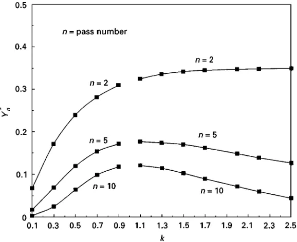
n. The optimal zone lengths YH1n for maximum solute removalFn(YH1n) inn-passes were obtained as follows. First,CMn(Z,Y1n) was obtained from eqns (1) and (2) numerically withMsections and with the use of eqns (3) and (4) as well as the given value ofY1n. Fn(Y1n) was then calculated from eqns (9) and (10) andRnally,YH1nwas obtained from the requirement,
dFn(Y1n)/dY1n"0.
The optimal values ofYH1nare shown inFigure 3 as a function ofk with pass numbern.
Constant Optimum Zone Length in Each Pass
Figure 2 Numerical values of the optimal variable zone length for each pass.
Figure 3 Numerical values of the constant optimum zone length for all passes.
Separation Theory in Analogue
Simulators
Zone Re\ning Simulator fork(1
Zone reVning region, 0)x)(L!l ) Figure 5
shows a zone reRning simulator fork(1. The ingot is operated by an array of vertical tubes, such as
Figure 4 Numerical values of the constant optimal zone length for each pass.
Figure 5 Hand-operated liquid-level zone refining simulator fork(1. The areaazof the zone tube determines the value ofk that is operated, in accordance with:
az"ma(1!k)
K [12]
The liquid level in tubeiafter thenth pass is:
hn i"
(m!1)ahn
i\1#ahnm\#1i\1#azhni\1
ma#az
,
i"1,2,N!m [13]
Figure 6 Hand-operated liquid-level zone refining simulator fork'1. i"N!(m!1),N!(M!2),2,N!1
[14]
A zone pass is performed by continuously readjust-ing the cross-sectional area of the zone tube accordreadjust-ing to eqn (14) after closing each rearmost tube. At the end of each pass the total amount of the liquid in the zone tube can readily be forced into the last tube, which is then closed as the zone leaves the ingot.
The liquid level in tubeiafter thenth pass is:
hn i"
(N!i)a#az,i (N!i)a#az,i ,
i"N!m#1,N!m#2,2,N!1
[15]
Zone-re\ning Simulator fork'1
Zone-reVning region, 0)x)(L!l ) Figure 6
shows a zone-reRning simulator fork'1, in which
empty:
az"ma(k!1)
k [16]
The liquid level in tubeiafter thenth pass is:
hn i"
(m!1)ahn
i\1#ahnm\#1i\1!azhni\1
ma!az
,
i"1,2,N!m [17]
Normal-freezing region, (L!l )4x4L It is well known that the cross-sectional areaaz,i of the zone tube for k'1 in this section of ingot, (L!l))x)L, must be readjusted continuously after closing each rearmost tube.
The liquid level in tubeiafter thenth pass is:
hn i"
(N!i)a!az,i (N!i)a!az,i
hn
i\1,
Further Reading
Bertein F (1958) Simple analogue apparatus for study of treatment of an ingot by zone melting.Journal of Phys-ics in Radium19: 121A.
Bertein F (1958) Electrical analogue for study of treatment of an ingot by zone melting. Journal of Physics in Radium19: 182A
Davies LW (1959) The efRciency of zone reRning processes. Transactions of the American Institute of Mechanical Engineers215: 672.
Ho CD, Yeh HM and Yeh TL (1997) Multipass zone reRning with speciRed ingot volume of frustum with sine-function proRle.Separation and PuriTcation Tech-nology11: 57}63.
Ho CD, Yeh HM, Yeh TL and Sheu HW (1997) Simulation of multipass zone reRning processes within whole ingot.
Journal of the Chinese Institute of Chemical Engineers 28: 271}279.
Ho CD, Yeh HM and Yeh TL (1998) Numerical analysis on optimal zone lengths for each pass in multipass zone reRning processes.Canadian Journal of Chemical Engineers76: 113}119.
Ho CD, Yeh HM and Yeh TL (1999) The optimal variation of zone lengths in multipass zone reRning processes. Separation and PuriTcation Technology76: 113}119. Lawson WD, and Nielsen S (1962) In: Schoen HM (ed.)
New Chemical Engineering Separation Techniques. New York: John Wiley and Sons Inc.
Lord NW (1953) Analysis of molten-zone reRning. Trans-actions of the American Institute of Mechanical Engineers197: 1531.
Pfann WG (1964)Zone Melting, 2nd edn. New York: John Wiley and Sons Inc.
DISTILLATION
Azeotropic Distillation
F. M. Lee and R. W. Wytcherley,
GTC Technology Corporation, Houston, Texas, USA Copyright^ 2000 Academic Press
Introduction
An azeotrope occurs when the composition of a va-pour in equilibrium with a liquid mixture has the same composition as the liquid. Azeotropic distillation takes advantage of azeotropes that form naturally between many components. Azeotropic distillation involves the formation of an azeotrope, or the use of an existing azeotrope, to effect a desired separation.
For almost 100 years the existence of naturally occurring azeotropes has been used to purify chem-icals. In 1902, Young reported using benzene as an azeotropic agent to dehydrate ethanol. This Rrst in-dustrial application was in a batch mode and there-fore not conducive to widespread commercial use. Twenty years elapsed before a continuous commer-cial process was developed. In 1923, Backus, Keyes and Stevens of the United States, and Guinot of France developed continuous azeotropic distillation processes for the dehydration of ethanol. As with Young’s batch process, the continuous processes re-lied upon the ethanol}benzene}water ternary azeo-tropic mixture for dehydrating ethanol. From that time, azeotropic distillation processes have grown to become an indispensable tool in today’s industries.
Desirable properties for an azeotropic entrainer are:
1. Heterogeneous azeotrope for ease of entrainer re-covery
2. Commercially available and inexpensive 3. Nontoxic
4. Chemically stable 5. Noncorrosive
6. Low latent heat of vaporization
7. Low viscosity to provide high tray efRciencies 8. Low freezing point to allow ease of handling and
storage
Azeotropic distillation is an essential unit operation in today’s processes. Applications using azeotropic distillation are readily apparent in the chemical pro-cess industry (CPI), speciality chemicals and food industries. Applications from various industries are listed inTable 1.
The main advantages of azeotropic distillation are in allowing the separation of chemicals that cannot feasibly be separated by conventional distillation, such as systems containing azeotropes or pinch points, and improving the economics of the separ-ation by saving energy and increasing recovery. The main disadvantages of azeotropic distillation are the larger diameter column required to allow for in-creased vapour volume due to the azeotropic agent, and an increase in control complications compared with simple distillation.