Sentiment Classification using Automatically Extracted Subgraph Features

Proceedings of the NAACL HLT 2010 Workshop on Computational Approaches to Analysis and Generation of Emotion in Text, pages 131–139,

Sentiment Classification using Automatically Extracted Subgraph Features

Shilpa Arora, Elijah Mayfield, Carolyn Penstein-Ros´e and Eric Nyberg

Language Technologies Institute Carnegie Mellon University

5000 Forbes Avenue, Pittsburgh, PA 15213

{shilpaa, emayfiel, cprose, ehn}@cs.cmu.edu

Abstract

In this work, we propose a novel representa-tion of text based on patterns derived from lin-guistic annotation graphs. We use a subgraph mining algorithm to automatically derive fea-tures as frequent subgraphs from the annota-tion graph. This process generates a very large number of features, many of which are highly correlated. We propose a genetic program-ming based approach to feature construction which creates a fixed number of strong classi-fication predictors from these subgraphs. We evaluate the benefit gained from evolved struc-tured features, when used in addition to the bag-of-words features, for a sentiment classi-fication task.

1 Introduction

In recent years, the topic of sentiment analysis has been one of the more popular directions in the field of language technologies. Recent work in super-vised sentiment analysis has focused on innovative approaches to feature creation, with the greatest im-provements in performance with features that in-sightfully capture the essence of the linguistic con-structions used to express sentiment, e.g. (Wilson et al., 2004), (Joshi and Ros´e, 2009)

In this spirit, we present a novel approach that leverages subgraphs automatically extracted from linguistic annotation graphs using efficient subgraph mining algorithms (Yan and Han, 2002). The diffi-culty with automatically deriving complex features comes with the increased feature space size. Many of these features are highly correlated and do not

provide any new information to the model. For ex-ample, a feature of typeunigram POS (e.g.

“cam-era NN”) doesn’t provide any additional

informa-tion beyond the unigram feature (e.g. “camera”), for words that are often used with the same part of speech. However, alongside several redundant fea-tures, there are also features that provide new infor-mation. It is these features that we aim to capture.

In this work, we propose an evolutionary ap-proach that constructs complex features from sub-graphs extracted from an annotation graph. A con-stant number of these features are added to the un-igram feature space, adding much of the represen-tational benefits without the compurepresen-tational cost of a drastic increase in feature space size.

In the remainder of the paper, we review prior work on features commonly used for sentiment anal-ysis. We then describe the annotation graph rep-resentation proposed by Arora and Nyberg (2009). Following this, we describe the frequent subgraph mining algorithm proposed in Yan and Han (2002), and used in this work to extract frequent subgraphs from the annotation graphs. We then introduce our novel feature evolution approach, and discuss our experimental setup and results. Subgraph features combined with the feature evolution approach gives promising results, with an improvement in perfor-mance over the baseline.

2 Related Work

the bag of words approach. Arora et al. (2009) show that deep syntactic scope features constructed from transitive closure of dependency relations give sig-nificant improvement for identifying types of claims in product reviews. Gamon (2004) found that using deep linguistic features derived from phrase struc-ture trees and part of speech annotations yields sig-nificant improvements on the task of predicting sat-isfaction ratings in customer feedback data. Wilson et al. (2004) use syntactic clues derived from depen-dency parse tree as features for predicting the inten-sity of opinion phrases1.

Structured features that capture linguistic patterns are often hand crafted by domain experts (Wilson et al., 2005) after careful examination of the data. Thus, they do not always generalize well across datasets and domains. This also requires a signif-icant amount of time and resources. By automati-cally deriving structured features, we might be able to learn new annotations faster.

Matsumoto et al. (2005) propose an approach that uses frequent sub-sequence and sub-tree mining ap-proaches (Asai et al., 2002; Pei et al., 2004) to derive structured features such as word sub-sequences and dependency sub-trees. They show that these features outperform bag-of-words features for a sentiment classification task and achieve the best performance to date on a commonly-used movie review dataset. Their approach presents an automatic procedure for deriving features that capture long distance depen-dencies without much expert intervention.

However, their approach is limited to sequences or tree annotations. Often, features that combine several annotations capture interesting characteris-tics of text. For example, Wilson et al. (2004), Ga-mon (2004) and Joshi and Ros´e (2009) show that a combination of dependency relations and part of speech annotations boosts performance. The anno-tation graph represenanno-tation proposed by Arora and Nyberg (2009) is a formalism for representing sev-eral linguistic annotations together on text. With an annotation graph representation, instances are rep-resented as graphs from which frequent subgraph patterns may be extracted and used as features for learning new annotations.

1_{Although, in this work we are classifying sentences and not}

phrases, similar clues may be used for sentiment classification in sentences as well

In this work, we use an efficient frequent sub-graph mining algorithm (gSpan) (Yan and Han, 2002) to extract frequent subgraphs from a linguis-tic annotation graph (Arora and Nyberg, 2009). An annotation graph is a general representation for ar-bitrary linguistic annotations. The annotation graph and subgraph mining algorithm provide us a quick way to test several alternative linguistic representa-tions of text. In the next section, we present a formal definition of the annotation graph and a motivating example for subgraph features.

3 Annotation Graph Representation and

Feature Subgraphs

Arora and Nyberg (2009) define the annotation graph as a quadruple: G = (N, E,Σ, λ), where N is the set of nodes, E is the set of edges, s.t. E ⊂ N ×N, andΣ = ΣN ∪ΣE is the set of la-bels for nodes and edges. λ : N ∪E → Σ is the labeling function for nodes and edges. Examples of node labels (ΣN) aretokens (unigrams)and annota-tions such aspart of speech,polarityetc. Examples of edge labels (ΣE) areleftOf,dependency typeetc.

TheleftOf relation is defined between two adjacent

nodes. Thedependency typerelation is defined be-tween a head word and its modifier.

Annotations may be represented in an annotation graph in several ways. For example, a dependency triple annotation ‘good amod movie’, may be repre-sented as ad amodrelation between the head word ‘movie’ and its modifier ‘good’, or as a noded amod

with edges ParentOfGov and ParentOfDep to the head and the modifier words. An example of an an-notation graph is shown in Figure 1.

The instance in Figure 1 describes a movie review comment, ‘interesting, but not compelling.’. The words ‘interesting’ and ‘compelling’ both have pos-itive prior polarity, however, the phrase expresses negative sentiment towards the movie. Heuristics for special handling ofnegationhave been proposed in the literature. For example, Pang et al. (2002) ap-pend every word following a negation, until a punc-tuation, with a ‘NOT’ . Applying a similar technique to our example gives us two sentiment bearing fea-tures, one positive (‘interesting’) and one negative

(‘NOT-compelling’), and the model may not be as

positive and negative sentiment present.

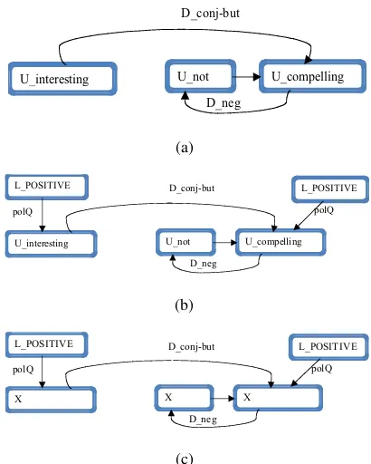
In Figure 2, we show three discriminating sub-graph features derived from the annotation sub-graph in Figure 1. These subgraph features capture the nega-tive sentiment in our example phrase. The first fea-ture in 2(a) capfea-tures the pattern using dependency relations between words. A different review com-ment may use the same linguistic construction but with a different pair of words, for example“a pretty

good, but not excellent story.”This is the same

lin-guistic pattern but with different words the model may not have seen before, and hence may not clas-sify this instance correctly. This suggests that the feature in 2(a) may be too specific.

In order to mine general features that capture the rhetorical structure of language, we may add prior polarity annotations to the annotation graph, us-ing a lexicon such as Wilson et al. (2005). Fig-ure 2(b) shows the subgraph in 2(a) with polar-ity annotations. If we want to generalize the pat-tern in 2(a) to any positive words, we may use the feature subgraph in Figure 2(c) withX wild cards on words that are polar or negating. This feature subgraph captures the negative sentiment in both phrases ‘interesting, but not compelling.’ and “a

pretty good, but not excellent story.”. Similar

gener-alization using wild cards on words may be applied with other annotations such as part of speech anno-tations as well. By choosing where to put the wild card, we can get features similar to, but more pow-erful than, the dependency back-off features in Joshi and Ros´e (2009).

U_interesting U_, U_but U_not U_compelling U_. D_conj-but

D_neg

L_POSITIVE _{L_POSITIVE}

polQ polQ

posQ P_VBN

posQ P_,

posQ P_CC

posQ P_RB

posQ P_JJ

posQ P_.

Figure 1: Annotation graph for sentence‘interesting, but not compelling.’ . Prefixes: ‘U’ for unigrams (tokens), ‘L’ for po-larity, ‘D’ for dependency relation and ‘P’ for part of speech. Edges with no label encode the ‘leftOf’ relation between words.

4 Subgraph Mining Algorithms

In the previous section, we demonstrated that sub-graphs from an annotation graph can be used to

iden-U_interesting U_not U_compelling D_conj-but

D_neg

(a)

U_interesting U_not U_compelling D_conj-but

D_neg

L_POSITIVE L_POSITIVE polQ polQ

(b)

X X X

D_conj-but

D_neg

L_POSITIVE L_POSITIVE

polQ polQ

(c)

Figure 2: Subgraph features from the annotation graph in Figure 1

tify the rhetorical structure used to express senti-ment. The subgraph patterns that represent general linguistic structure will be more frequent than sur-face level patterns. Hence, we use a frequent sub-graph mining algorithm to find frequent subsub-graph patterns, from which we construct features to use in the supervised learning algorithm.

The goal in frequent subgraph mining is to find frequent subgraphs in a collection of graphs. A graphG′ _{is a subgraph of another graphGif there}

exists a subgraph isomorphism2 from G′ _toG,

de-noted byG′_⊑G.

Earlier approaches in frequent subgraph mining (Inokuchi et al., 2000; Kuramochi and Karypis, 2001) used a two-step approach of first generating the candidate subgraphs and then testing their fre-quency in the graph database. The second step in-volves a subgraph isomorphism test, which is NP-complete. Although efficient isomorphism testing algorithms have been developed making it practical to use, with lots of candidate subgraphs to test, it can

2

still be very expensive for real applications.

gSpan (Yan and Han, 2002) uses an alternative

pattern growth based approach to frequent subgraph mining, which extends graphs from a single sub-graph directly, without candidate generation. For each discovered subgraphG, new edges are added recursively until all frequent supergraphs ofGhave been discovered. gSpan uses a depth first search tree (DFS) and restricts edge extension to only vertices on the rightmost path. However, there can be multi-ple DFS trees for a graph. gSpan introduces a set of rules to select one of them as representative. Each graph is represented by its unique canonical DFS code, and the codes for two graphs are equivalent if the graphs are isomorphic. This reduces the compu-tational cost of the subgraph mining algorithm sub-stantially, making gSpan orders of magnitude faster than other subgraph mining algorithms. With sev-eral implementations available 3_{, gSpan has been} commonly used for mining frequent subgraph pat-terns (Kudo et al., 2004; Deshpande et al., 2005). In this work, we use gSpan to mine frequent subgraphs from the annotation graph.

5 Feature Construction using Genetic Programming

A challenge to overcome when adding expressive-ness to the feature space for any text classification problem is the rapid increase in the feature space size. Among this large set of new features, most are not predictive or are very weak predictors, and only a few carry novel information that improves classification performance. Because of this, adding more complex features often gives no improvement or even worsens performance as the feature space’s signal is drowned out by noise.

Riloff et al. (2006) propose a feature subsump-tion approach to address this issue. They define a hierarchy for features based on the information they represent. A complex feature is only added if its discriminative power is a delta above the discrimi-native power of all its simpler forms. In this work, we use a Genetic Programming (Koza, 1992) based approach which evaluates interactions between

fea-3

http://www.cs.ucsb.edu/˜xyan/software/ gSpan.htm, http://www.kyb.mpg.de/bs/people/ nowozin/gboost/

tures and evolves complex features from them. The advantage of the genetic programing based approach over feature subsumption is that it allows us to eval-uate a feature using multiple criteria. We show that this approach performs better than feature subsump-tion.

A lot of work has considered this genetic pro-gramming problem (Smith and Bull, 2005). The most similar approaches to ours are taken by Kraw-iec (2002) and Otero et al. (2002), both of which use genetic programming to build tree feature represen-tations. None of this work was applied to a language processing task, though there has been some sim-ilar work to ours in that community, most notably (Hirsch et al., 2007), which built search queries for topic classification of documents. Our prior work (Mayfield and Ros´e, 2010) introduced a new feature construction method and was effective when using unigram features; here we extend our approach to feature spaces which are even larger and thus more problematic.

The Genetic Programming (GP) paradigm is most advantageous when applied to problems where there is not a correct answer to a problem, but instead there is a gradient of partial solutions which incre-mentally improve in quality. Potential solutions are represented as trees consisting of functions (non-leaf nodes in the tree, which perform an action given their child nodes as input) and terminals (leaf nodes in the tree, often variables or constants in an equa-tion). The tree (an individual) can then be inter-preted as a program to be executed, and the output of that program can be measured for fitness (a mea-surement of the program’s quality). High-fitness in-dividuals are selected for reproduction into a new generation of candidate individuals through a breed-ing process, where parts of each parent are combined to form a new individual.

present.

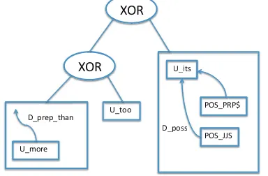
The tree in Figure 3 is a simplified example of our evolved features. It combines three features, a uni-gram feature ‘too’ (centre node) and two subgraph features: 1) the subgraph in the leftmost node oc-curs in collocations containing “more than” (e.g.,

“nothing more than”or“little more than”), 2) the subgraph in the rightmost node occurs in negative phrases such as “opportunism at its most glaring”

(JJS is a superlative adjective and PRP$ is a pos-sessive pronoun). A single feature combining these weak indicators can be more predictive than any part alone.

!"#$

!"#$

%&'(($

%&)(*+$ ,&-*+-&'./0$

%&1'2$

3"4&3#35$

3"4&664$ ,&-(22$

%&1'2 %&1

3"4&3#35$&3#

3"4&664$ 3"4&66 ,&-(22(22

Figure 3: A tree constructed using subgraph features and GP (Simplified for illustrative purposes)

In the rest of this section, we first describe the feature construction process using genetic program-ming. We then discuss how fitness of an individual is measured for our classification task.

5.1 Feature Construction Process

We divide our data into two sets, training and test. We again divide our training data in half, and train our GP features on only one half of this data4This is to avoid overfitting the final SVM model to the GP features. In a single GP run, we produce one feature to match each class value. For a sentiment classifica-tion task, a feature is evolved to be predictive of the positive instances, and another feature is evolved to be predictive of the negative documents. We repeat this procedure a total of 15 times (using different seeds for random selection of features), producing a total of 30 new features to be added to the feature space.

4

For genetic programming we used the ECJ toolkit (http://cs.gmu.edu/˜eclab/projects/ecj/).

5.2 Defining Fitness

Our definition of fitness is based on the concepts of precision and recall, borrowed from informa-tion retrieval. We define our set of documents as being comprised of a set of positive documents

P0, P1, P2, ...P_u and a set of negative documents

N0, N1, N2, ...Nv. For a given individualIand doc-umentD, we definehit(I, D)to equal 1 if the state-mentIis true of that document and 0 otherwise. Pre-cision and recall of an individual feature for predict-ing positive documents5is then defined as follows:

P rec(I) =

u

X

i=0

hit(I, Pi)

u

X

i=0

hit(I, Pi) + v

X

i=0

hit(I, Ni) (1)

Rec(I) =

u

X

i=0

hit(I, Pi)

u (2)

We then weight these values to give significantly more importance to precision, using theFβmeasure, which gives the harmonic mean between precision and recall:

Fβ(I) =

(1 +β2

)×(P rec(I)×Rec(I)) (β2_{×P rec(I)) +Rec(I)} (3)

In addition to this fitness function, we add two penalties to the equation. The first penalty applies to prevent trees from becoming overly complex. One option to ensure that features remain moderately simple is to simply have a maximum depth beyond which trees cannot grow. Following the work of Otero et al. (2002), we penalize trees based on the number of nodes they contain. This discourages bloat, i.e. sections of trees which do not contribute to overall accuracy. This penalty, known as parsimony pressure, is labeledPPin our fitness function.

The second penalty is based on the correlation be-tween the feature being constructed, and the sub-graphs and unigrams which appear as nodes within that individual. Without this penalty, a feature may

5_{Negative precision and recall are defined identically, with}

often be redundant, taking much more complexity to represent the same information that is captured with a simple unigram. We measure correlation us-ing Pearson’s product moment, defined for two vec-torsX,Y as:

ρx,y =

E[(X−µX)(Y −µY)]

σXσY

(4)

This results in a value from 1 (for perfect align-ment) to -1 (for inverse alignalign-ment). We assign a penalty for any correlation past a cutoff. This func-tion is labeledCC(correlation constraint) in our fit-ness function.

Our fitness function therefore is:

Fitness=F1 8 +

P P +CC (5)

6 Experiments and Results

We evaluate our approach on a sentiment classifi-cation task, where the goal is to classify a movie review sentence as expressing positive or negative sentiment towards the movie.

6.1 Data and Experimental Setup

Data: The dataset consists of snippets from Rot-ten Tomatoes (Pang and Lee, 2005) 6. It consists of 10662 snippets/sentences total with equal num-ber positive and negative sentences (5331 each). This dataset was created and used by Pang and Lee (2005) to train a classifier for identifying positive sentences in a full length review. We use the first 8000 (4000 positive, 4000 negative) sentences as training data and evaluate on remaining 2662 (1331 positive, 1331 negative) sentences. We added part of speech and dependency triple annotations to this data using the Stanford parser (Klein and Manning, 2003).

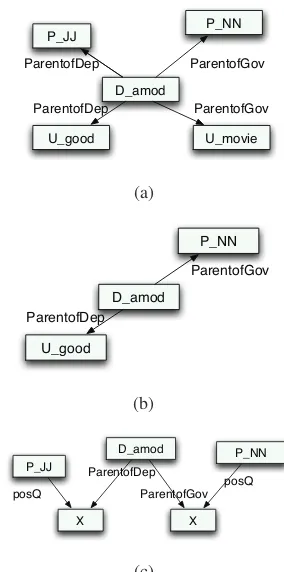
Annotation Graph: For the annotation graph rep-resentation, we usedUnigrams (U),Part of Speech (P)andDependency Relation Type (D)as labels for the nodes, andParentOfGovandParentOfDepas la-bels for the edges. For a dependency triple such as “amod good movie”, five nodes are added to the an-notation graph as shown in Figure 4(a).

ParentOf-Gov and ParentOfDep edges are added from the

6

http://www.cs.cornell.edu/people/pabo/ movie-review-data/rt-polaritydata.tar.gz

D_amod

U_good

P_JJ P_NN

U_movie ParentofGov

ParentofGov ParentofDep

ParentofDep

(a)

D_amod

U_good

P_NN

ParentofGov

ParentofDep

(b)

D_amod

X P_JJ

P_NN

X posQ ParentofGov ParentofDep

posQ

(c)

Figure 4: Annotation graph and a feature subgraph for dependency triple annotation “amod good camera”. (c) shows an alternative representation with wild cards

dependency relation node D amod to the unigram nodes U good and U movie. These edges are also added for the part of speech nodes that correspond to the two unigrams in the dependency relation, as shown in Figure 4(a). This allows the algorithm to find general patterns, based on a dependency rela-tion between two part of speech nodes, two unigram nodes or a combination of the two. For example, a subgraph in Figure 4(b) captures a general pat-tern wheregoodmodifies a noun. This feature ex-ists in “amod good movie”, “amod good camera” and other similar dependency triples. This feature is similar to the the dependency back-off features pro-posed in Joshi and Ros´e (2009).

adding more edges. However, with lots of edges, the complexity of the subgraph mining algorithm and the number of subgraph features increases tremen-dously.

Classifier: For our experiments we use Support

Vector Machines (SVM) with a linear kernel. We use the SVM-light7 implementation of SVM with default settings.

Parameters:ThegSpanalgorithm requires setting

the minimum support threshold (minsup) for the subgraph patterns to extract. Support for a subgraph is the number of graphs in the dataset that contain the subgraph. We experimented with several values for minimum support andminsup = 2gave us the best performance.

For Genetic Programming, we used the same pa-rameter settings as described in Mayfield and Ros´e (2010), which were tuned on a different dataset8 than one used in this work, but it is from the same movie review domain. We also consider one alter-ation to these settings. As we are introducing many new and highly correlated features to our feature space through subgraphs, we believe that a stricter constraint must be placed on correlation between features. To accomplish this, we can set our correla-tion penalty cutoff to 0.3, lower than the 0.5 cutoff used in prior work. Results for both settings are re-ported.

Baselines: To the best of our knowledge, there is

no supervised machine learning result published on this dataset. We compare our results with the fol-lowing baselines:

• Unigram-only Baseline:In sentiment analysis,

unigram-only features have been a strong base-line (Pang et al., 2002; Pang and Lee, 2004). We only use unigrams that occur in at least two sentences of the training data same as Mat-sumoto et al. (2005). We also filter out stop words using a small stop word list9_.

• χ2

Baseline: For our training data, after

filter-ing infrequent unigrams and stop words, we get

7_{http://svmlight.joachims.org/} 8_{Full movie review data by Pang et al. (2002)} 9

http://nlp.stanford.edu/ IR-book/html/htmledition/

dropping-common-terms-stop-words-1.html (with one modification: removed ‘will’, added ‘this’)

8424 features. Adding subgraph features in-creases the total number of features to44,161, a factor of 5 increase in size. Feature selec-tion can be used to reduce this size by select-ing the most discriminative features.χ2

feature selection (Manning et al., 2008) is commonly used in the literature. We compare two methods of feature selection withχ2

, one which rejects features if theirχ2

score is not significant at the 0.05 level, and one that reduces the number of features to match the size of our feature space with GP.

• Feature Subsumption (FS):Following the idea

in Riloff et al. (2006), a complex feature C is discarded if IG(S) ≥ IG(C) − δ, where IG is Information Gain and S is a simple feature that representationally

sub-sumes C, i.e. the text spans that match S

are a superset of the text spans that match C. In our work, complex features are sub-graph features and simple features are uni-gram features contained in them. For example,

(D amod) Edge P arentOf Dep(U bad) is a complex feature for whichU bad is a sim-ple feature. We tried same values for δ ∈ {0.002,0.001,0.0005}, as suggested in Riloff et al. (2006). Since all values gave us same number of features, we only report a single re-sult for feature subsumption.

• Correlation (Corr): As mentioned earlier,

some of the subgraph features are highly corre-lated with unigram features and do not provide new knowledge. A correlation based filter for subgraph features can be used to discard a com-plex featureCif its absolute correlation with its simpler feature (unigram feature) is more than a certain threshold. We use the same threshold as used in the GP criterion, but as a hard filter instead of a penalty.

6.2 Results and Discussion

Settings #Features Acc. ∆

Uni 8424 75.66

-Uni + Sub 44161 75.28 -0.38 Uni + Sub,χ2

sig. 3407 74.68 -0.98 Uni + Sub,χ2

size 8454 75.77 +0.11 Uni + Sub, (FS) 18234 75.47 -0.19 Uni + Sub, (Corr) 18980 75.24 -0.42 Uni + GP (U)† 8454 76.18 +0.52 Uni + GP (U+S)‡ 8454 76.48 +0.82 Uni + GP (U+S)† 8454 76.93 +1.27

Table 1: Experimental results for feature spaces with un-igrams, with and without subgraph features. Feature se-lection with 1) fixed significance level (χ2_{sig.), 2) fixed}

feature space size (χ2_{size), 3) Feature Subsumption (FS)}

and 4) Correlation based feature filtering (Corr)). GP fea-tures for unigrams only{GP(U)}, or both unigrams and subgraph features {GP(U+S)}. Both the settings from Mayfield and Ros´e (2010) (‡) and more stringent correla-tion constraint (†) are reported. #F eaturesis the num-ber of features in the training data. Accis the accuracy and∆is the difference from unigram only baseline. Best performing feature configuration is highlighted in bold.

than the unigram-only approach. With GP, we ob-serve a marginally significant gain (p <0.1) in per-formance over unigrams, calculated using one-way ANOVA. Benefit from GP is more when subgraph features are used in addition to the unigram features, for constructing more complex pattern features. Ad-ditionally, our performance is improved when we constrain the correlation more severely than in previ-ously published research, supporting our hypothesis that this is a helpful way to respond to the problem of redundancy in subgraph features.

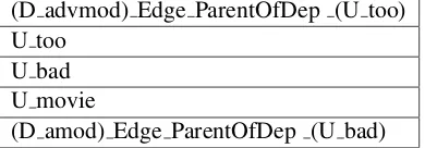
A problem that we see withχ2

feature selection is that several top ranked features may be highly cor-related. For example, the top 5 features based onχ2 score are shown in Table 2; it is immediately obvi-ous that the features are highly redundant.

With GP based feature construction, we can sider this relationship between features, and con-struct new features as a combination of selected un-igram and subgraph features. With the correlation criterion in the evolution process, we are able to build combined features that provide new informa-tion compared to unigrams.

The results we present are for the best

perform-(D advmod) Edge ParentOfDep (U too) U too

U bad U movie

(D amod) Edge ParentOfDep (U bad)

Table 2: Top features based onχ2_score

ing parameter configuration that we tested, after a series of experiments. We realize that this places us in danger of overfitting to the particulars of this data set, however, the data set is large enough to partially mitigate this concern.

7 Conclusion and Future Work

We have shown that there is additional information to be gained from text beyond words, and demonstrated two methods for increasing this information -a subgr-aph mining -appro-ach th-at finds common syn-tactic patterns that capture sentiment-bearing rhetor-ical structure in text, and a feature construction technique that uses genetic programming to com-bine these more complex features without the redun-dancy, increasing the size of the feature space only by a fixed amount. The increase in performance that we see is small but consistent.

In the future, we would like to extend this work to other datasets and other problems within the field of sentiment analysis. With the availability of several off-the-shelf linguistic annotators, we may add more linguistic annotations to the annotation graph and richer subgraph features may be discovered. There is also additional refinement that can be performed on our genetic programming fitness function, which is expected to improve the quality of our features.

Acknowledgments

This work was funded in part by the DARPA Ma-chine Reading program under contract FA8750-09-C-0172, and in part by NSF grant DRL-0835426. We would like to thank Dr. Xifeng Yan and Marisa Thoma for the gSpan code.

References

Re-views. Proceedings of the HLT/NAACL.

Shilpa Arora and Eric Nyberg. 2009. Interactive Anno-tation Learning with Indirect Feature Voting. Proceed-ings of the HLT/NAACL (Student Research Work-shop).

Tatsuya Asai, Kenji Abe, Shinji Kawasoe, Hiroshi Sakamoto and Setsuo Arikawa. 2002. Efficient sub-structure discovery from large semi-sub-structured data. Proceedings of SIAM Int. Conf. on Data Mining (SDM).

Mukund Deshpande , Michihiro Kuramochi , Nikil Wale and George Karypis. 2005. Frequent Substructure-Based Approaches for Classifying Chemical Com-pounds. IEEE Transactions on Knowledge and Data Engineering.

Michael Gamon. 2004. Sentiment classification on cus-tomer feedback data: noisy data, large feature vec-tors, and the role of linguistic analysis, Proceedings of COLING.

Laurence Hirsch, Robin Hirsch and Masoud Saeedi. 2007. Evolving Lucene Search Queries for Text Clas-sification. Proceedings of the Genetic and Evolution-ary Computation Conference.

Mahesh Joshi and Carolyn P. Ros´e. 2009. Generalizing Dependency Features for Opinion Mining. Proceed-ings of the ACL-IJCNLP Conference (Short Papers). Akihiro Inokuchi, Takashi Washio and Hiroshi Motoda.

2000. An Apriori-based Algorithm for Mining Fre-quent Substructures from Graph Data. Proceedings of PKDD.

Dan Klein and Christopher D. Manning. 2003.Accurate unlexicalized parsing. Proceedings of the main con-ference of the ACL.

John Koza. 1992. Genetic Programming: On the Pro-gramming of Computers by Means of Natural Selec-tion. MIT Press.

Krzysztof Krawiec. 2002. Genetic programming-based construction of features for machine learning and knowledge discovery tasks. Genetic Programming and Evolvable Machines.

Taku Kudo, Eisaku Maeda and Yuji Matsumoto. 2004. An Application of Boosting to Graph Classification. Proceedings of NIPS.

Michihiro Kuramochi and George Karypis. 2002. Fre-quent Subgraph Discovery. Proceedings of ICDM. Christopher D. Manning, Prabhakar Raghavan and

Hin-rich Schtze. 2008. Introduction to Information Re-trieval. Proceedings of PAKDD.

Shotaro Matsumoto, Hiroya Takamura and Manabu Oku-mura. 2005. Sentiment Classification Using Word Sub-sequences and Dependency Sub-trees. Proceed-ings of PAKDD.

Elijah Mayfield and Carolyn Penstein-Ros´e. 2010. Using Feature Construction to Avoid Large Feature Spaces in Text Classification. Proceedings of the Ge-netic and Evolutionary Computation Conference. Fernando Otero, Monique Silva, Alex Freitas and Julio

Nievola. 2002. Genetic Programming for Attribute Construction in Data Mining. Proceedings of the Ge-netic and Evolutionary Computation Conference. Bo Pang, Lillian Lee and Shivakumar Vaithyanathan.

2002. Thumbs up? Sentiment Classication using Ma-chine Learning Techniques. Proceedings of EMNLP. Bo Pang and Lillian Lee. 2004. A Sentimental

Educa-tion: Sentiment Analysis Using Subjectivity Summa-rization Based on Minimum Cuts. Proceedings of the main conference of ACL.

Bo Pang and Lillian Lee. 2005.Seeing stars: Exploiting class relationships for sentiment categorization with respect to rating scales. Proceedings of the main con-ference of ACL.

Jian Pei, Jiawei Han, Behzad Mortazavi-asl, Jianyong Wang, Helen Pinto, Qiming Chen, Umeshwar Dayal and Mei-chun Hsu. 2004. Mining Sequential Pat-terns by Pattern-Growth: The PrefixSpan Approach. Proceedings of IEEE Transactions on Knowledge and Data Engineering.

Ellen Riloff, Siddharth Patwardhan and Janyce Wiebe. 2006. Feature Subsumption for Opinion Analysis. Proceedings of the EMNLP.

Matthew Smith and Larry Bull. 2005.Genetic Program-ming with a Genetic Algorithm for Feature Construc-tion and SelecConstruc-tion. Genetic Programming and Evolv-able Machines.

Theresa Wilson, Janyce Wiebe and Rebecca Hwa. 2004. Just How Mad Are You? Finding Strong and Weak Opinion Clauses. Proceedings of AAAI.

Theresa Wilson, Janyce Wiebe and Paul Hoff-mann. 2005. Recognizing Contextual Polarity in Phrase-Level Sentiment Analysis. Proceedings of HLT/EMNLP.