UNCORRECTED PR
OOF
1
Randomized parcellation based inference
2Q1
Benoit
Da Mota
a,b,⁎
,1, Virgile Fritsch
a,b,1, Gaël Varoquaux
a,b, Tobias Banaschewski
e,f, Gareth J. Barker
d,
3
Arun L.W. Bokde
j,k, Uli Bromberg
g, Patricia Conrod
d,h, Jürgen Gallinat
i, Hugh Garavan
j,s,t, Jean-Luc Martinot
l,m,
4Frauke Nees
e,f, Tomas Paus
n,o,p, Zdenka Pausova
r, Marcella Rietschel
e,f, Michael N. Smolka
q, Andreas Ströhle
i,
5Vincent Frouin
b, Jean-Baptiste Poline
b,c, Bertrand Thirion
a,b,⁎
,
the IMAGEN consortium
26 a
Parietal Team, INRIA Saclay-Île-de-France, Saclay, France
7 b
CEA, DSV, I2
BM, Neurospin bât 145, 91191 Gif-Sur-Yvette, France 8Q2 c
Henry H. Wheeler Jr. Brain Imaging Center, University of California at Berkeley, USA
9 d
Institute of Psychiatry, Kings College London, UK 10 eCentral Institute of Mental Health, Mannheim, Germany
11 f
Medical Faculty Mannheim, University of Heidelberg, Germany
12 g
Universitaetsklinikum Hamburg Eppendorf, Hamburg, Germany
13 h
Department of Psychiatry, Universite de Montreal, CHU Ste. Justine Hospital, Canada
14 i
Department of Psychiatry and Psychotherapy, Campus Charité Mitte, Charité Universitätsmedizin Berlin, Germany 15Q3 j
Q4 Institute of Neuroscience, School of Medicine, Trinity College Dublin, Dublin, Ireland
16 k
Discipline of Psychiatry, School of Medicine, Trinity College Dublin, Dublin, Ireland
17Q5 lInstitut National de la Santé et de la Recherche Médicale, INSERM CEA Unit 1000“Imaging & Psychiatry”, University Paris Sud, Orsay, Maison de Solenn, University Paris Descartes, Paris, France
18 m
AP-HP Department of Adolescent Psychopathology and Medicine, Maison de Solenn, University Paris Descartes, Paris, France
19 n
Rotman Research Institute, University of Toronto, Toronto, Canada
20 o
School of Psychology, University of Nottingham, UK
21 p
Montreal Neurological Institute, McGill University, Canada
22 q
Neuroimaging Center, Department of Psychiatry and Psychotherapy, Technische Universität Dresden, Germany 23 rThe Hospital for Sick Children, University of Toronto, Toronto, Canada
24Q6 sDepartment of Psychiatry, University of Vermont, USA
25 t
Department of Psychology, University of Vermont, USA Q7
26
27
a b s t r a c t
a r t i c l e i n f o
28 Article history:
29 Accepted 5 November 2013 30 Available online xxxx 31
32 33
34 Keywords: 35 Group analysis 36 Parcellation 37 Reproducibility 38 Multiple comparisons 39 Permutations
40 Neuroimaging group analyses are used to relate inter-subject signal differences observed in brain imaging with
41 behavioral or genetic variables and to assess risks factors of brain diseases. The lack of stability and of sensitivity
42 of current voxel-based analysis schemes may however lead to non-reproducible results. We introduce a new
43 approach to overcome the limitations of standard methods, in which active voxels are detected according to
44 a consensus on several random parcellations of the brain images, while a permutation test controls the false
45 positive risk. Both on synthetic and real data, this approach shows higher sensitivity, better accuracy and higher
46 reproducibility than state-of-the-art methods. In a neuroimaging–genetic application, wefind that it succeeds in
47 detecting a significant association between a genetic variant next to theCOMTgene and the BOLD signal in the
48 left thalamus for a functional Magnetic Resonance Imaging contrast associated with incorrect responses of the
49 subjects from aStop Signal Taskprotocol.
50 © 2013 Elsevier Inc. All rights reserved.
51 52 53
54
55 Introduction
56 Analysis of brain images acquired on a group of subjects makes it 57 possible to draw inferences on regionally-specific anatomical properties
58 of the brain, or its functional organization. The major difficulty with
59 such studies lies in the inter-subject variability of brain shape and
60 vasculature. In functional studies, a task-related variability of subject
61 performance is also observed. The standard-analytic approach is to
62 register and normalize the data in a common reference space. However
63 a perfect voxel-to-voxel correspondence cannot be attained, and the
64 impact of anatomical variability is tentatively reduced by smoothing
65 (Frackowiak et al., 2003). This problem holds for any statistical test,
in-66 cluding those associated with multivariate procedures. In the absence of
67 ground truth, choosing the best procedure to analyze the data is a
chal-68 lenging problem. Practitioners as well as methodologists tend to prefer NeuroImage xxx (2013) xxx–xxx
⁎ Corresponding authors at: CEA, DSV, I2
BM, Neurospin bât 145, 91191 Gif-Sur-Yvette, France.
E-mail addresses:[email protected](B. Da Mota),[email protected] (B. Thirion).
1
These authors contributed equally to this work.
2URL:http://www.imagen-europe.com
1053-8119/$–see front matter © 2013 Elsevier Inc. All rights reserved. http://dx.doi.org/10.1016/j.neuroimage.2013.11.012
Contents lists available atScienceDirect
NeuroImage
UNCORRECTED PR
OOF
69 models that maximize the sensitivity of a test under a given control for70 false detections. The level of sensitivity conditional to this control is in-71 deed informative on the usefulness of a model.
72 Classic statistical tests for neuroimaging
73 The reference approach in neuroimaging is tofit and test a model 74 at each voxel (univariate voxelwise method), but the large number of 75 tests performed yields a multiple comparison problem. The statistical 76 significance of the voxel intensity test can be corrected with various sta-77 tistical procedures. First, Bonferroni correction consists in adjusting the 78 significance threshold by dividing it by the number of tests performed. 79 This approach is known to be conservative, especially when non-80 independent tests are involved, which is the case of neighboring voxels 81 in neuroimaging. Another approach consists in a permutation test to 82 perform a family-wise correction of the p-values (Nichols and Holmes, 83 2002). Although computationally costly, this method has been shown 84 to yield more sensitive results than studies involving Bonferroni-85 corrected experiments (Petersson et al., 1999). A good compromise be-86 tween computation cost and sensitivity can be found in analytic correc-87 tions based on Random Field Theory (RFT), in which the smoothness of 88 the images is estimated (Worsley et al., 1992). However, this approach 89 requires both high threshold and data smoothness to be really effective 90 (Hayasaka et al., 2004).
91 Another widely used method is a test on cluster size, which aims 92 to detect spatially extended effects (Friston et al., 1993; Poline and 93 Mazoyer, 1993; Roland et al., 1993). The statistical significance of the 94 size of an activation cluster can be obtained with theoretical corrections 95 based on the RFT (Hayasaka et al., 2004; Worsley et al., 1996b) or with a 96 permutation test (Holmes et al., 1996; Nichols and Holmes, 2002). 97 Cluster-size tests tend to be more sensitive than voxel-intensity tests, 98 especially when the signal is spatially extended (Friston et al., 1996; 99 Moorhead et al., 2005; Poline et al., 1997), at the expense of a strong sta-100 tistical control on all the voxels within such clusters. This approach 101 however suffers from several drawbacks. First, such a procedure is in-102 trinsically unstable and its result depends strongly on an arbitrary 103 cluster-forming threshold (Friston et al., 1996). The threshold-free 104 cluster enhancement (TFCE) addresses this issue, by avoiding the 105 choice of an explicit,fixed threshold (Salimi-Khorshidi et al., 2011; 106 Smith and Nichols, 2009) but leads to other arbitrary choices: the 107 TFCE statistic mixes cluster-extent and cluster-intensity measures in 108 proportions that can be defined by the user. More generally, tests 109 that combine cluster size and voxel intensity have been proposed 110 (Hayasaka and Nichols, 2004; Poline et al., 1997). Second, the correla-111 tion between neighboring voxels varies across brain images, which 112 makes detection difficult where the local smoothness is low. Combin-113 ing permutations and RFT to adjust for spatially-varying smoothness 114 leads to more sensitive procedures (Hayasaka et al., 2004; Salimi-115 Khorshidi et al., 2011). A more complete discussion of the limitations 116 and comparisons of these techniques can be found in (Moorhead 117 et al., 2005; Petersson et al., 1999).
118 Spatial models for group analysis in neuroimaging
119 Spatial models try to overcome the lack of correspondence between 120 individual images at the voxel level. The most straightforward and 121 widely used technique consists of smoothing the data to increase the 122 overlap between subject-specific activated regions (Worsley et al., 123 1996a). In the literature, several approaches propose more elaborate 124 techniques to model the noise in neuroimaging, like Markov Random 125 Fields (Ou et al., 2010), wavelet decomposition (Ville et al., 2004), spa-126 tial decomposition or topographic methods (Flandin and Penny, 2007; 127 Friston and Penny, 2003) and anatomically informed models (Keller 128 et al., 2009). These techniques are not widely used probably because 129 they are computationally costly and not always well-suited for analysis 130 of a group of subjects. A popular approach consists of working with
131 subject-specific Regions of Interest (ROIs), that can be defined in a
132 way that accommodates inter-subject variability (Nieto-Castanon
133 et al., 2003). The main limitation of such an approach (Bohland et al.,
134 2009) is that there is no widely accepted standard for partitioning the
135 brain, especially for the neocortex. Data-driven parcellation was
pro-136 posed byThirion et al. (2006)to overcome this limitation: they improve
137 the sensitivity of random effect analysis by considering parcels defined
138 at the group level.
139
Neuroimaging–genetic studies
140 While most studies investigate the difference of activity between
141 groups or the level of activity within a population, neuroimaging
142 studies are often concerned by testing the effect of exogeneous
vari-143 ables on imaging target variables, and there is increasing interest
144 in the joint study of neuroimaging and genetics to improve
under-145 standing of both normal and pathological variability of the brain
orga-146 nization. Single nucleotide polymorphisms (SNPs) are the most
147 common genetic variants used in such studies: They are numerous
148 and represent approximately 90% of the genetic between-subject
vari-149 ability (Collins et al., 1998). Voxel intensity and cluster size methods
150 have been used for genome-wide association studies (GWAS) (Stein
151 et al., 2010), but the multiple comparison problem does not permit
152
finding significant results, despite efforts to estimate the effective 153 number of tests (Gao et al., 2010) or by running computationally
154 expensive, but accurate permutation tests (Da Mota et al., 2012).
Re-155 cently, important efforts have been done to design more sophisticated
156 multivariate methods (Floch et al., 2012; Kohannim et al., 2011;
157 Vounou et al., 2010), the results of which are more difficult to
inter-158 pret; another alternative is to work at the gene level instead of SNPs
159 (Ge et al., 2012; Hibar et al., 2011).
160 The randomized parcellation approach
161 The parcellation model (Thirion et al., 2006) has several advantages:
162 (i) it is a simple and easily interpretable method, (ii) by reducing the
163 number of descriptors, it reduces the multiple comparisons problem,
164 and (iii) the choice of the parcellation algorithm can lead to parcels
165 adapted to the local smoothness. But parcellations, when considered
166 as spatial functions, highly depend on the data used to construct them
167 and the choice of the number of parcels. In general, a parcellation
de-168
fined in a given context might not be a good descriptor in a slightly 169 different context, or may generalize poorly to new subjects. This implies
170 a lack of reproducibility of the results across subgroups, as illustrated
171 later inFig. 7. The weakness of this approach is the large impact of a
172 parcellation scheme that cannot be optimized easily for the sake of
sta-173 tistical inference; it may thus fail to detect effects in poorly segmented
174 regions. We propose to solve this issue by using several randomized
175 parcellations (Bühlmann et al., 2012; Varoquaux et al., 2012) generated
176 using resampling methods (bootstrap) and average the corresponding
177 statistical decisions. Replacing an estimator such as parcel-level
infer-178 ence by means of bootstrap estimates is known tostabilizeit; a fortunate
179 consequence is that thereproducibilityof the results (across subgroups
180 of subjects) is improved. Formally, this can be understood as handling
181 the parcellation as a hidden variable that needs to be integrated out in
182 order to obtain the posterior distribution of statistical values. Thefinal
183 decision is taken with regard to the stability of the detection of a voxel
184 (Alexander and Lange, 2011; Meinshausen and Bühlmann, 2010) across
185 parcellations, compared to the null hypothesis distribution obtained by
186 a permutation test.
187 A multivariate problem: the detection of outliers
188 The benefits of the randomized parcellation approach can also be
ob-189 served in multivariate analysis procedures, such as predictive modeling
UNCORRECTED PR
OOF
191 the latter: neuroimaging datasets often contain atypical observations;192 suchoutlierscan result from acquisition-related issues (Hutton et al.,
193 2002), bad image processing (Wu et al., 1997), or they can merely be ex-194 treme examples of the high variability observed in the population. 195 Because of the high dimensionality of neuroimaging data, screening 196 the data is very time consuming, and becomes prohibitive with large 197 cohort studies. Covariance-based outlier detection methods have 198 been proposed to perform statistically-controlled inclusion of subjects 199 in neuroimaging studies (Fritsch et al., 2012) and yield a good detection 200 accuracy. These methods rely on prior reduction of the data dimen-201 sion which is obtained by taking signal averages within predefined 202 brain parcels. As a consequence, the results depend on afixed brain 203 parcellation and are unstable. Randomization might thus improve 204 the procedure.
205 Outline
206 In“Materials and methods”, we introduce methodological prerequi-207 sites and we describe the randomized parcellation approach. In 208 “Experiments”, we provide the description of the experiments used to as-209 sess the performances of our procedure. We evaluate our approach on 210 simulations and on real fMRI data for the random effect analysis problem. 211 Then, we illustrate the interest of the approach for neuroimaging–genetic 212 studies, on a gene candidate (COMT) which is widely investigated in 213 the context of brain diseases. Finally, we show that this technique is 214 suitable for detecting outliers in neuroimaging data, thus extending 215 the application scope of randomized parcellations to multivariate 216 analysis procedures. In“Results”, we report the results of the experi-217 ments andfinally we discuss different aspects and choices that can in-218Q8 fluence the method performance.
219 Materials and methods
220 Statistical modeling for group studies
221 Neuroimaging studies are often designed to test the effect of miscel-222 laneous variables on imaging target variables. For a study involvingn 223 subjects, neuroscientists generally consider the following model:
Y¼Xβþ;
224
225 whereYis an×pmatrix representing the signal ofnsubjects de-226 scribed each bypdescriptors (e.g. voxels or parcels of an fMRI contrast 227 image) andXis then× (q1+q2) set ofq1explanatory variables, a 228 predefined linear combination of which is to be tested for a non-zero 229 effect, andq2covariables that explain some portion of the signal but 230 are not to be tested for an effect.βare the coefficients of the model 231 to be estimated, andis some Gaussian noise. Variables inXcan be 232 of any type (genetic, artificial, behavioral, experimental…). A standard 233 univariate analysis technique consists infittingpOrdinary Least Square 234 (OLS) regressions, one for each column ofY, as a target variable, and 235 each time perform a non-zero significance test on thecTβquantity, 236 wherec∈ℝq1þq2is thecontrast vectorthat defines the linear
combina-237 tion of the variables to be tested. This test involves the estimated coef-238 ficients of the modelβ^and the noise estimateσ^to compute a standard 239 t- orF-statistic.
240 Parcellation and Ward algorithm
241 In functional neuroimaging, brain atlases are often used to provide 242 a low-dimensional representation of the data by considering signal 243 averages within groups of voxels (regions of interest). If those groups 244 of voxels do not overlap and every voxel belongs to one group, 245 the termparcelis employed, and the atlas is called aparcellation. 246 In this work, we restrict ourselves to working with parcellations, 247 although our methodology could be applied to any kind of brain
248 partition (set of ROIs). We construct parcellations from the images
249 that we work on, because this data-driven approach better takes into
250 account the unknown spatial data structure. Following (Michel et al.,
251 2012; Varoquaux et al., 2012), we use spatially-constrained Ward
252 hierarchical clustering (Ward, 1963) to cluster the voxels inKparcels,
253 yielding what we will refer to as aK-parcellation. This approach
cre-254 ates a hierarchy of parcels represented as a tree. The root of the tree
255 is the unique parcel that gathers all the voxels, the leaves being the
256 parcels with only one voxel. When merging two clusters, the Ward
257 criterion chooses the cluster that produces a supra-cluster with
mini-258 mal variance. Any cut of the tree corresponds to a unique parcellation.
259 This algorithm has several advantages: (i) It captures well local
corre-260 lations into spatial clusters, (ii) efficient implementations exist
261 (Pedregosa et al., 2011), and (iii) obtained parcellations are invariant
262 by permutation of the subjects and sign of the input data. A gives a
263 formal description of Ward's clustering algorithm. We also show
264 some examples of parcellations and discuss the geometric properties
265 of the parcels.
266 Randomized parcellation based inference
267
Randomized parcellation based inference(RPBI) performs several
268 standard analyses based on different parcellations and aggregates the
269 corresponding statistical decisions. LetPbe afinite set of parcellations,
270 andVbe the set of voxels under consideration. Given a voxelvand a
271 parcellationP, the parcel-based thresholding functionθtis defined as:
θtðv;PÞ ¼
1 if FðΦPð ÞvÞNt
0 otherwise
ð1Þ
272 273 whereΦP:V→Pis a mapping function that associates each voxel
274 with a parcel from the parcellationP(∀v∈P(i),Φ
P(v) =P(i)). For 275 a predefined test,Freturns theF-statistic associated with the
aver-276 age signal of a given parcel (ator other statistic is also possible).
277 Finally, the aggregating statistic at a voxelvis given by the counting
278 functionCt:
Ctðv;PÞ ¼
X
P∈P
θtðv;PÞ: ð2Þ
279 280
Ctðv;PÞrepresents the number of times the voxelvwas part of a parcel
281 associated with a statistical value larger thantacross the folds of the
282 analysis conducted on the set of parcellationsP. We set the parameter
283
tto ensure a Bonferroni-corrected control atpb0.13in each of the 284 parcel-level analyses. In practice, the results are weakly sensitive to
285 mild variations oft. In order to assess the significance of the counting
286 statistic at each voxel, we perform a permutation test, i.e. we tabulate
287 the distribution ofCtðv;PÞunder the null hypothesis that there is no
sig-288 nificant correlation between the voxels' mean signal and the target
289 variable. Depending on the comparison to be performed, we switch
290 labels (comparison between groups) or we swap signs (testing that
291 the mean is non-zero). As a result, we get a voxel-wise p-value map
292 similar to a standard group analysis map (seeFig. 1). We obtain
293 family-wise error control by tabulating the maximal value across voxels
294 in the permutation procedure. Theθtfunction can be replaced by any
295 function that is convex with respect tot. In particular, the natural choice
296
θt(v,P) =F(ΦP(v)) yields similar results (not shown in the paper) but 297 its computation requires much more memory since thev→θt(v,P)
298 mapping and bootstrap averages are no longer sparse. An important
299 prerequisite for our approach is to generate several parcellations that
300 are different enough from each other to guarantee that the analysis
3
We determine this value empirically to obtain a well-behaved null distribution of the counting statistic. With 1 target and 1000 parcels, it corresponds to a raw p-valueb10−4
UNCORRECTED PR
OOF
301 conducted with each of those parcellations samples correctly the set of 302 regions that display some activation for the effect considered. One way 303 to achieve this is to take bootstrap samples of subjects and apply Ward's 304 clustering algorithm to their contrast maps, to build brain parcellations 305 that best summarize the data subsamples, i.e. so that the parcel-level 306 mean signal summarizes the signal within each parcel, in each subject. 307 If enough subjects are used, all the parcellations offer a good represen-308 tation of the whole dataset. It is important that the bootstrap scheme 309 generates parcellations with enough entropy (Varoquaux et al.,
310 2012). Spatial models try to address the problem of imperfect voxel-311 to-voxel correspondence after coregistration of the subjects in the 312 same reference space. Our approach is clearly related to anisotropic 313 smoothing (Sol et al., 2001), in the sense that obtained parcels are 314 not spherical and in the aggregation of the signals of voxels in a 315 given parcel, certain directions are preferred. Unlike smoothing or spa-316 tial modeling applied as a preprocessing, our statistical inference em-317 beds the spatial modeling in the analysis and decreases the number 318 of tests and their dependencies. In addition to the expected increase 319 of sensitivity, the randomization of the parcellations ensures a better 320 reproducibility of the results, unlike inference on one fixed 321 parcellation. Last, theCtðv;PÞstatistic is reliable in the sense that is
322 does not depend on side effects such as the parcel size. This is formally 323 checked inAppendix B.
324 Sensitivity and accuracy assessments
325 We want to assess the sensitivity of our approach at afixed level of 326 specificity and compare it to the other methods. Thus, we are interested 327 in whether or not a significant effect was reported according to the dif-328 ferent methods. Under the assumption that the method specificity is 329 controlled with a given false positive rate, the method with the highest 330 number of detections is the most sensitive.
331 Note that a direct comparison of the sensitivity of the different pro-332 cedures (voxel-level, cluster-level, TFCE, parcel-based), i.e. their rate of 333 detections, is not very meaningful. Indeed, only voxel-level statistics 334 provide a strong control on false detections. The other procedures 335 violate the subset pivotality condition, namely that the rejection of 336 the null at a given location does not alter the distribution of the deci-337 sion statistics under the null at other locations (see e.g.Westfall and
338 Troendle, 2008). This means that the rejection of the null at a given
339 location is not independent of the rejection at the null at nearby
340 locations; specifically, the rejection of the null at a given voxel is
341 bound to the voxel in voxel-based tests, while it is not for other kinds
342 of inferences considered here. Strictly speaking, those only reject a
343 global null. Note however, that such a weak control on false detections
344 is still useful in problems with small effect sizes (see“Neuroimaging–
345 genetic study”). The ideal method would be able to detect small effects,
346 but would be also quite specific about their location. That is why an
347 analysis of the sensitivity should always be considered with an analysis
348 of the accuracy.
349 In our experiments, to estimate a method's accuracy, we construct
350 Receiver Operating Characteristic (ROC) curves (Hanley and McNeil,
351 1982) by reporting the proportion of true positives in the detections
352 for different levels of false positives. The true/false positives are
deter-353 mined according to aground truththat is defined based on the
simula-354 tion setup or empirically when dealing with real data. In practice, we
355 are interested in low false positive rates, so we present the ROC curves
356 in logarithmic scale.
357 Use of randomized parcellation in multivariate models
358 Various neuroimaging methods rely on a prior dimension reduction
359 of the data, and can therefore benefit from a randomized parcellation
360 approach that stabilizes the ensuing statistical procedure. Beyond the
361 specific case of group analysis investigated in this manuscript, we
362 apply the randomized parcellation technique to the outlier detection
363 task. Unlike group analysis, outlier detection can be formulated as a
364 multivariate problem, especially because we consider
covariance-365 based outlier detection (Fritsch et al., 2012), where an estimate of the
366 data covariance matrix is computed and then used to provide an outlier
367 score for each observation, i.e. correlations between features are taken
368 into account in thefinal decision about whether or not an image should
369 be considered an outlier.
370
IMAGEN, a neuroimaging–genetic study
371 IMAGEN is a European multicentric study involving adolescents
[image:4.595.52.535.55.294.2]UNCORRECTED PR
OOF
373 database with fMRI associated with 99 different contrast images for374 4 protocols in more than 2000 subjects, who gave informed signed 375 consent. Regarding the functional neuroimaging data, the faces pro-376 tocol (Grosbras and Paus, 2006) was used, with the [angry faces–
377 control] contrast, i.e. the difference between watching angry faces
378 and non-biological stimuli (concentric circles). We also use the 379 Stop Signal Task protocol (Logan, 1994) (SST), with the activation 380 during a [go wrong] event, i.e. when the subject pushes the wrong 381 button. Images from the Modified Incentive Delay task (Knutson 382 et al., 2000) (MID) were used to construct alternative randomized 383 parcellations.
384 Eight different 3 T scanners from multiple manufacturers (GE, 385 Siemens, Philips) were used to acquire the data. Standard preprocessing, 386 including slice timing correction, spike and motion correction, temporal 387 detrending (functional data), and spatial normalization (anatomical 388 and functional data), were performed using the SPM8 software 389 and its default parameters; functional images were resampled at 390 3 mm resolution. All images were warped in the MNI152 coordinate 391 space using a study-specific template. Obvious outliers detected using 392 simple rules such as large registration or segmentation errors 393 or very large motion parameters were removed after this step. 394 BOLD time series was recorded using Echo-Planar Imaging, with 395 TR = 2200 ms, TE = 30 ms,flip angle = 75∘and spatial resolution 396 3 mm × 3 mm × 3 mm. Gaussian smoothing at 5 mm-FWHM wasfi -397 nally added.4Contrasts were obtained using a standard linear model, 398 based on the convolution of the time course of the experimental con-399 ditions with the canonical hemodynamic response function, together 400 with standard high-passfiltering (period = 120 s) and temporally 401 auto-regressive noise model. The estimation of thefirst-level was car-402 ried out using the SPM8 software. T1-weighted MPRAGE anatomical 403 images were acquired with spatial resolution 1 mm × 1 mm × 1 mm, 404 and gray matter probability maps were available for 1986 subjects as 405 outputs of the SPM8“New Segmentation”algorithm applied to the 406 anatomical images. A mask of the gray matter was built by averaging 407 and thresholding the individual gray matter probability maps. More 408 details about data preprocessing can be found in (Thyreau et al., 409 2012). Genotyping was performed genome-wide using Illumina 410 Quad 610 and 660 chips, yielding approximately 600,000 autosomic 411 SNPs. 477,215 SNPs are common to the two chips and passplink stan-412 dard parameters (Minor Allele FrequencyN0.05, Hardy–Weinberg 413 EquilibriumPb0.001, missing rate per SNPN0.05).
414 Experiments
415 Random effect analysis on simulated data
416 We simulate fMRI contrast images as volumes of shape 40 × 40 × 417 40 voxels. Each contrast image contains a simulated 4 × 4 × 4 activa-418 tion patch at a given location, with a spatial jitter following a three-419 dimensional N(0,I3) distribution (coordinates of the jitter are rounded 420 to the nearest integers). The strength of the activation is set so that 421 the signal to noise ratio (SNR) peaks at 2 in the most associated 422 voxel. The background noise is drawn from a (0,1) distribution, 423 Gaussian-smoothed atσnoiseisotropic and normalized by its global 424 empirical standard deviation. After superimposing noise and signal 425 images, we optionally smooth atσpost= 2.12 voxels isotropic, corre-426 sponding to a 5 voxel Full Width at Half Maximum (FWHM). Voxels 427 with a probability above 0.1 to be active in a large sample test are 428 considered as part of the ground truth. Ten subsamples (or groups) 429 of 20 images are then generated to perform analyses. Each time,
430 RPBI was conducted with one hundred 1000-parcellations built from
431 a bootstrapped selection of the 20 images involved. For each of the
432 10 groups, we expect to obtain a p-value map that shows a significant
433 effect at the mean location of generated artificial activations in the
434 contrast images.
435 We investigate the ability of four methods to actually recover the
436 region of activation:
437 (i) voxel-level group analysis, which is the standard method in
neu-438 roimaging;
439 (ii) cluster-size group analysis, which is known to be more sensitive
440 than voxel-intensity group analysis;
441 (iii) threshold-free cluster enhancement (TFCE) (Smith and Nichols,
442 2009);
443 (iv) RPBI, which is our contribution.
444 445 We control the specificity of each procedure by permutation testing.
446 In order to ensure an accurate type 1 error control, we generate 400 sets
447 of 20 images with no activation (i.e. the images are only noise with
448
σnoise= 1, and SNR = 0). We evaluate the false positive rate at
449 voxel level for RPBI. We perform the same simulated data experiment
450 with a more complex activation shape (shown inFig. 2) as we think it
451 better corresponds to activations encountered in real data. The rest of
452 the experimental design remains the same and we perform the same
453 comparison between methods.
454 Random effect analysis on real fMRI data
455 In this experiment, we work with an [angry faces–control] fMRI
456 contrast. We kept data from 1430 subjects after removal of the
457 subjects with missing data and/or bad or missing covariables. After
458 standard preprocessing of the images, including registration of the
459 subjects onto the same template, we test each voxel for a zero mean
460 across the 1430 subjects with an OLS regression, including
handed-461 ness and sex as covariables, yielding a reference voxel-wise p-value
462 map. We threshold this map in order to keep 5% of the most active
463 voxels (corresponding to−log10PN77.5), and we consider it the
464 ground truth. Since we use a voxel based threshold, the ground
465 truth may be biased to voxel-level statistics (thus disadvantaging
466 our method).
467 Our objective is to retrieve the population's reference activity
468 pattern on subsamples of 20 randomly drawn subjects and compare
469 the performance of several methods in this problem. Because of the
re-470 duced number of subjects used, we cannot expect to retrieve the same
471 activation map as in the full-sample analysis due to a loss in statistical
4
[image:5.595.332.535.557.699.2]Smoothing is applied only in thefirst-level analysis in order to improve the sensitivity of the General Linear Model that yields the contrast maps.
UNCORRECTED PR
OOF
472 power. We therefore measure the sensitivity and we build ROC curves473 to assess the performance of the methods. We perform our experiment 474 on 10 different subsamples and we use the same analysis methods as 475 the previous experiment. We propose to observe the behavior of our 476 method with the use of parcellations of different kinds. We perform 477 analysis of the 10 different subsamples with the following parcellation 478 schemes:
479 (i) RPBI (sh. parcels) with parcellations built on bootstrapped sub-480 samples of 150 images among the 1430 images corresponding 481 to the fMRI contrast under study;
482 (ii) RPBI (alt. parcels) with shared parcellations built on images 483 corresponding to another, independent fMRI contrast;
484 (iii) RPBI (rand. parcels) with shared parcellations built on smoothed 485 Gaussian noise;
486
487 We also assess the stability of all these methods by counting how 488 many times each voxel was associated to a significant effect across 489 subsamples. We present the inverted cumulative normalized histogram 490 of this count for each method, restricting our attention to the voxels 491 that were reported at least once. A method is considered to be more 492 stable than another if the same voxels appear more often, that is if its 493 histogram shows many high values.
494 Neuroimaging–genetic study
495 The aim of this experiment is to show that RPBI has the potential to 496 uncover new relationships between neuroimaging and genetics. We 497 consider an fMRI contrast corresponding to events where subjects 498 make motor response errors ([go wrong] fMRI contrast from a Stop Sig-499 nal Task) and its associations withSingle-Nucleotide Polymorphisms 500 (SNPs) in the COMT gene. This gene codes for the Catechol-O-501 methyltransferase, an enzyme that catalyzes transfer of neurotransmit-502 ters like dopamine, epinephrine and norepinephrine, making it one of 503 the most studied genes in relation to brain (Puls et al., 2009; Smolka 504 et al., 2007). Subjects with too many missing voxels in the brain mask 505 or with bad task performance were discarded. Regarding genetic vari-506 ants, we kept 27 SNPs in theCOMTgene (±20 kb) that passplink stan-507 dard parameters (Minor Allele FrequencyN0.05, Hardy–Weinberg 508 Equilibrium PN0.001, missing rate per SNPb0.05). The ± 20 kb 509 window includes some SNPs in the ARVCF gene, that are inlinkage
510 disequilibriumwith SNPs inCOMT. Age, sex, handedness and acquisition
511 center were included in the model as confounding variables. Remaining
512 missing data were replaced by the median over the subjects for the
cor-513 responding variables. After applying all exclusion criteria 1372 subjects
514 remained for analysis.
515 For each of the 27 SNPs, we perform a massively univariate
voxel-516 wise analysis with the algorithm presented in (Da Mota et al., 2012),
517 including cluster-size analysis (Hayasaka and Nichols, 2003), and
518 RPBI through 100 different Ward's 1000-parcellations. To assess
sig-519 nificance with a good degree of confidence we performed 10,000
520 permutations.
521 Outlier detection
522 Wefinally apply the concept of randomized parcellations to
out-523 lier detection. We work with a cohort of 1886 fMRI contrast images.
524 In afirst step, we randomly select 300 subjects and summarize the
525 dataset by computing a 500-parcellation (obtained by Ward's) and
526 averaging signal over each parcel. We perform a reference outlier
de-527 tection on this dataset with a regularized version of a robust
covari-528 ance estimatorRMCD-RP(Fritsch et al., 2012). This outlier detection
529 algorithm consists offitting robust covariance estimators to random
530 data projections. For the outlier detection we use the average of the
531 Mahalanobis distances of the observations to the population mean
532 in every projection subspace. In a second step, we perform outlier
de-533 tections with RMCD-RP on random subsamples: We randomly draw
534 a subsample ofnsubjects and perform 100 outlier detections with
535 RMCD-RP on 100 different p-dimensional representations of the
536 data defined by 100 Ward'sp-parcellations built on 300 bootstrapped
537 subjects from the whole cohort. Following the model of RPBI, we
re-538 port how many times each subject was reported as an outlier through
539 these 100 outlier detections and we use that number as an outlier
540 score. We hence construct two Receiver Operating Characteristic
541 (ROC) curves (Hanley and McNeil, 1982): one for randomized
542 parcellation-based (RPB) outlier detection and the other as the
aver-543 age ROC curve of the 100 inner outlier detections used to obtain the
544 RPB outlier detection. Finally, we report the rate of correct detections
545 when 5% of false detections are accepted, to control the sensitivity of
546 this test when wrongly rejecting few non-outlier data. These statistics
547 make it possible to easily measure the accuracy improvement of RPB
548 outlier detection across several experiments performed with different
549 subsamples ofnsubjects (keeping the same reference decision
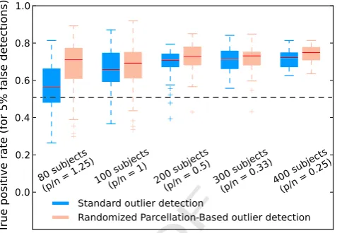
ob-550 tained at thefirst step). In our experiment, we choose to work with
[image:6.595.62.529.512.704.2]a
b
Fig. 3.Simulated data (cubic effect). ROC curves for various analysis methods across 10 random subsamples containing 20 subjects. SNR = 2 and noise spatial smoothness: (a)σnoise= 0,
(b)σnoise= 1. The curves are obtained by thresholding the statistical brain maps at various levels, yielding as many points on the curves. Thex-axis is the expected number of false
positives per image. The curve for cluster-size inference could not be built forσnoise= 0 because the detections correspond either to true positives only, or to false positives only. RPBI
UNCORRECTED PR
OOF
551 p= 100 andn= {80,100,200,300,400}, yieldingp/nconfigurations552 that correspond to various problem difficulties. For afixed (n,p) couple, 553 we run the experiment on 50 different subsamples and we present the 554 rate of correct detections in a box-plot.
555 Results
556 Random effect analysis on simulated data
557 Voxel-intensity group analysis is the only method that benefits 558 from a posteriori smoothing, while spatial methods lose sensitivity 559 and accuracy when the images are smoothed. This is in agreement 560 with the theory and the results of (Worsley et al., 1996a).Figs. 3 561 and 4show that detections made by spatial methods (cluster-size 562 group analysis, TFCE and RPBI) do not come with wrongly reported 563 effects in voxels close to the actual effect location. This would be the 564 case for a method that simply extends a recovered effect to the neigh-565 boring voxels and would wrongly be thought to be more sensitive be-566 cause it points out more voxels. RPBI offers the best accuracy as its 567 ROC curve dominates inFig. 3. We could not always build ROC curves 568 for the size method. This illustrates an issue of the cluster-569 forming threshold: most voxels do not pass the threshold and then
570 were discarded by the method, leading to a true positive rate equal
571 to zero. The cluster-forming threshold directly acts on the recovery
572 capability of the method, but lowering the threshold does not increase
573 the sensitivity of this approach in general. By integrating over
multi-574 ple thresholds, the TFCE partially addresses this issue. We also
en-575 countered an issue in the construction of ROC curves for
voxel-576 intensity based analysis in our simulations with a complex-shaped
ac-577 tivation (seeFig. 4): either there were only true positives, or there
578 were only false positives in our results, hence a lack of point for the
579 construction of the ROC curves. When no signal is put in the data
580 (SNR = 0), RPBI reports an activation 37 times over 400 atPb0.1
581 FWER corrected, 20 times atPb0.05 FWER corrected, and 4 times
582 atPb0.01 FWER corrected. In all cases, it corresponds to the nominal
583 type I error rate.
584 Random effect analysis on real fMRI data
585 Fig. 5a shows the sensitivity improvement relative to cluster-size
586 for various analysis methods under control for false detections at
587 5% FWER. Cluster-size was taken as the reference because it is the
588 method that yields the most sensitivity among state-of-the-art
589 methods to which we compare RPBI to. RPBI achieves the best
[image:7.595.75.535.53.213.2]a
b
Fig. 4.Simulated data (complex activation shape). ROC curves for various analysis methods across 10 random subsamples containing 20 subjects. SNR = 2 and noise spatial smoothness: (a)σnoise= 0, (b)σnoise= 1. The curves are obtained by thresholding the statistical brain maps at various levels, yielding as many points on the curves. Thex-axis is the expected number
of false positives per image. The curve for cluster-size inference could not be built forσnoise= 0 because the detections correspond either to true positives only, or to false positives only.
For the same reason, voxel-intensity performance could not be presented in any of the plots. RPBI outperforms other methods.
a
b
Fig. 5.Real fMRI data. Evaluation of the performances for various analysis methods across 10 random subsamples containing 20 subjects, on a [angry faces–control] fMRI contrast from the facesprotocol. (a) Sensitivity improvement relative to cluster-size under control of the specificity at 5% FWER. (b) ROC curves built with a pseudo ground truth where 5% of the most active voxels across 1430 subjects are kept. RPBI and TFCE have similar performance for low false positive rates (b10−2
[image:7.595.63.545.531.712.2]UNCORRECTED PR
OOF
590 sensitivity improvement, and RPBI with shared, alternative or random591 parcels are always more sensitive than TFCE. Voxel-level group anal-592 ysis yields poor performance while cluster-size analysis is comparable 593 to TFCE. These gains in sensitivity should be linked with a measure 594 of accuracy (see“Materials and methods”).Fig. 5b shows the ROC 595 curves associated with the performance of the methods under com-596 parison. For acceptable levels of false positives (b10−2), RPBI almost 597 equals TFCE when we use parcellations that have been built on the 598 contrast under study. RPBI with alternative or random parcels yields 599 poor recovery although these approaches are based on the random-600 ized parcellation scheme. This demonstrates that the sensitivity is 601 not a sufficient criterion and that the choice of parcellations plays 602 an important role in the success of RPBI. Unlike simulations, real 603 data may contain outliers, which reduce the effectiveness of all 604 the presented methods. One benefit of RPBI with shared parcels is
605 that the impact of bad samples in the test set is lowered, because
606 the parcellations are informed by potentially abundant side data.
607 This requires other data from a similar protocol, butFig. 5b shows
608 that this approach outperforms other methods byfinding more true
609 positives.
610 The lack of stability of group studies is a well-known issue, yet it
de-611 pends on the analysis performed (Strother et al., 2002; Thirion et al.,
612 2007). RPBI has better reproducibility than the other methods, as
613 shown inFig. 7. The histogram of the RPBI method dominates, which
614 means that significant effects were reported more often at the same
lo-615 cation (i.e. the same voxel) across subgroups when using RPBI than
616 when using the other methods. For RPBI with shared parcels, it is even
617 more pronounced and this is explained by the fact that parcellations
618 are shared across subgroups, which is another advantage to this
619 method.
Voxel-level
Cluster-size
TFCE
RPBI
Reference
1.0
3.7
z=5
z=52
77.5
222
a)
subgroup no.1
1 0
4.0
z=-8
z=-18
77.5
222
[image:8.595.50.535.227.710.2]b)
subgroup no.2
Fig. 6.Negative logp-value associated with a non-zero intercept test with confounds (handedness, site, sex), on a [angry faces–control] fMRI contrast from thefacesprotocol. The subgroups maps are thresholded at−log10PN1 FWER corrected and the reference map at−log10PN77.5 (i.e. 5% of the most active voxels). Small activation clusters are surrounded with a blue
UNCORRECTED PR
OOF
620 In general, the same activation peaks rise from the cluster-size, the621 TFCE and the RPBI maps (seeFig. 6). The TFCE slightly improves the re-622 sults of cluster-size and provides voxel-level information. As can be seen 623 inFig. 6, the map returned by RPBI better matches the patterns of the 624 reference map and is less scattered. Voxel-based group analysis clearly 625 fails to detect some of the activation peaks.
626 Neuroimaging–genetic study
627 The SNP rs917478 yields the strongest correlation with the pheno-628 types and lies in an intronic region of ARVCF. The number of subjects 629 in each genotype group is balanced: 523 homozygous with major 630 allele, 663 heterozygous and 186 homozygous with minor allele. For 631 RPBI, 31 voxels (resp. 81) are significantly associated with that SNP 632 atPb0.05 FWER corrected (resp.Pb0.1) in the left thalamus, a re-633 gion involved in sensory-motor cognitive tasks. The association peak 634 has a p-value of 0.016 FWER corrected. Cluster-size inferencefinds 635 this effect but with a higher p-value (P= 0.046). Voxel-based infer-636 ence does notfind any significant effect. A significant association 637 for rs917479 is reported only by RPBI;Fig. 8shows that this SNP 638 is in high linkage disequilibrium (LD) with rs917478 (D′= 0.98 639 andR2= 0.96). As shown inFig. 8, those SNPs are also in LD with 640 rs9306235 and rs9332377 inCOMT, the targeted gene for this study. 641 Fig. 8shows the thresholded p-value maps obtained with RPBI with 642 rs917478.
643 The ARVCF gene has already been found to be associated with inter-644 mediate brain phenotypes and neurocognitive error tests in a study 645 about schizophrenia (Sim et al., 2012). We applied our method on this 646 gene, for which we have 33 SNPs, and did notfind any effect except 647 from rs917478 and SNPs in LD with it.
648 Outlier detection
649 Fig. 9illustrates the accuracy of RPB outlier detection as com-650 pared to standard outlier detection performed on data issued from 651 a single parcellation. We present the rate of correct detections 652 when 5% false detections are accepted. Since the experiment is con-653 ducted on 50 subsamples of n subjects, we present the results 654 for various values ofn(n∈{80,100,200,300,400}) with box-plots. 655 For a large number of subjects (low-dimensional settings: nbp) 656 RPB outlier detection performs slightly better than standard outlier 657 detection, while in high-dimensional settings (pNn) it clearly out-658 performs the classic approach. Relative results are the same when
659 allowing for any proportion of false detection comprising between
660 0% and 10%.
661
Discussion
662 In this work, we introduce a new method for statistical inference
663 on brain images (RPBI) based on a randomized version of the
664 parcellation model (Thirion et al., 2006) that is stabilized by a
boot-665 strap procedure. In both simulation and real data experiments, RPBI
666 shows better performance (sensitivity, recovery and reproducibility)
667 than standard methods. The strength of this method is that the
deci-668 sion statistic takes into account the spatial structure of the data. Also,
669 the randomization of the parcellations yields more reproducible
670 results in view of between-subject variability and lowers the effect of
671 inaccurate parcellation. Our experiments with simulated and real
672 data show that the choice of the parcellations can greatly influence
673 the success of RPBI. In this section, we discuss this choice. We also
674 discuss some factors that can influence the method performance,
675 such as images properties or tested features characteristics and
com-676 putational aspects.
677 Brain parcellations
678 In our experiments, we used Ward clustering to build brain
679 parcellations. The main advantage of this clustering algorithm is that
680 it has the ability to take into account spatial pattern similarities
be-681 tween a set of input images, which acts as a spatial regularization. In
682 addition, the Ward criteria is designed such that, taking the mean
sig-683 nal within each parcel as new features to describe one subject image
684 gives the optimal data representation in terms of preserved
informa-685 tion (for afixed dimension corresponding to the number of parcels).
686 Importantly, the variability of the parcellations is directly related to
687 the variability and number of the images on which they are built. We
688 determined empirically that using 1000 parcels is a good trade-off
be-689 tween accurate parcellations and dimension reduction. This choice
690 leads to using an average of 50 voxels per parcel, which is a good
691 order of magnitude to describe the activation clusters. Note that, this
692 number of parcels is far from standard brain atlases with, at best,
693 a few hundred ROIs, suggesting that atlases are not well-suited for
694 such studies. Ourfirst real data experiment demonstrates that it is
695 beneficial that the parcellations reflect the group spatial activity
696 pattern of the fMRI contrast under study: when the parcellations are
697 built on another fMRI contrast or on random noise, thefinal
perfor-698 mance of persistence analysis drops back to the level of
state-of-the-699 art methods in terms of accuracy.
700 RPBI and images properties
701 Ourfirst experiment shows that RPBI performance drops when
im-702 ages are smoothed a posteriori. Unlike voxel-intensity analysis,
703 cluster-size analysis, TFCE and RPBI, which are spatial methods, suffer
704 from data smoothing. In the presence of smooth noise, this experiment
705 also shows that RPBI outperforms other methods. Our experiment on
706 real data shows that RPBI can recover activations clusters of various
707 size and shape, as visible on the effect maps reported inFig. 6. Yet, the
708 use of parcels clearly helps in focusing on activations with a spatial
ex-709 tent of the order of the average parcel size. Cluster-size group analysis
710 also focuses more easily on some activations with a given size, according
711 to internal parameters such as the cluster forming threshold or an
op-712 tional data smoothing. TFCE is designed to address this issue and clearly
713 enhances the results of the cluster-size inference.
714 Sensitivity and reproducibility
715 Usually, the sensitivity of a procedure is compared under a given
716 control for false positives. Under this criterion, RPBI outperforms
Reproducibility across subgroups
[image:9.595.51.290.521.703.2]UNCORRECTED PR
OOF
RPBI
Cluster-size
Z=
4
Y=-19
X=-12
UNCORRECTED PR
OOF
717 voxel-intensity, cluster-size analysis and TFCE (Fig. 5.a). By aggregating718 100 × 1000 measurements, RPBI drastically reduces the multiple com-719 parison problem and stabilizes parcel-based statistics. Neuroimaging 720 studies are subject to a lack of reproducibility and using the most sensi-721 tive procedure does not guarantee the unveiling of reproducible results 722 (Strother et al., 2002; Thirion et al., 2007). Experiments on real data 723 show the gain in terms of reproducibility of RPBI compared to other 724 methods when the subset of subjects changes (Fig. 7). RPBI with shared 725 parcels has a better recovery and yields more reproducible results 726 across various analysis settings.
727 Randomized parcellation can be applied to various neuroimaging 728 tasks. However, sensitivity improvement is not straightforward and 729 may depend on problem-specific settings. In particular, our experiment 730 about outlier detection suggests that multivariate statistical algorithms 731 require a more subtle use of randomized parcellation in order to get sig-732 nificant sensitivity improvement.
733 Computational aspects
734 Our goal here is not to provide an exhaustive study of the computa-735 tional performance, but to report on our experience of the experiments 736 performed. The procedure is separated into two distinct steps: (i) the 737 generation of the 100 WardK-parcellations and extraction of the signal 738 means, then (ii) the statistical inference. The generation of parcellations 739 is optional (parcellations can be replaced by precomputed ones), but 740 Ward's hierarchical clustering algorithm is fast and this step takes 741 only a few minutes on a desktop computer for 100 parcellations. The 742 second step involves a permutation test. Our implementationfits a 743 Massively Univariate Linear Model (Da Mota et al., 2012; Stein et al., 744 2010) in an optimized version adapted to permutation testing and our 745 application. As a result, in our experiments with 20 subjects and 746 10,000 permutations, the statistical inference takes only 1 min × cores, 747 i.e. 5 s on a 12-core computer. The total computation time thus amounts 748 to a few minutes on a desktop computer and is limited by the construc-749 tion of the parcellations. Asymptotically, the computation time in-750 creases only linearly with the number of subjects and the number of 751 variables to test, which is a desirable property to scale to larger prob-752 lems like neuroimaging–genetic studies.
753 Conclusion
754 RPBI is a general detection method based on a consensus across 755 bootstrap estimates that can be applied to various neuroimaging prob-756 lems such as group analyses or outlier detection. In our work, we use 757 randomized parcellations to benefit from many ROI-based descriptions 758 of our datasets that we construct with Ward's clustering. Simulations 759 and real-data experiments show that RPBI is more sensitive and stable 760 than state-of-the-art analysis methods. This is the case for various 761 types of problems, including neuroimaging–genetic associations. We 762 also demonstrate that the RPBI framework can be applied to outlier de-763 tection problem and improves detections accuracy.
764 Acknowledgments
765 This work was supported by Digiteo grants (HiDiNim project and 766 ICoGeN project) and an ANR grant (ANR-10-BLAN-0128), as well the 767 Microsoft INRIA joint center grantA-brain.
768 The data were acquired within the IMAGEN project, which received 769 research funding from the E.U. Community's FP6,
LSHM-CT-2007-770 037286. This manuscript reflects only the authors' views and the
Com-771 munity is not liable for any use that may be made of the information
772 contained therein.
773
Appendix A. Formal description of Ward's clustering algorithm
774 Ward's clustering algorithm is a particular case ofhierarchical
775 agglomerative clustering(Johnson, 1967). LetY= {y1,…,yp}∈ℝn×p
776 be a set ofnfMRI volumes described bypvoxels each. For two clusters
777 of voxelscandc′, we define the distance:
Δc;c′¼j j þcj jcj jcj j′c′h iY c−h iY c′ 2
2; ðA:1Þ
778 779 whereh iYc¼j j1c∑j∈cy
j
. For each partitionC= {c1,…,ck} of the set of 780 voxelsY(i.e.∪c∈C=Yandci∩cj=Ø∀(ci,cj)∈C2), we noteC∗the
781 set of all pairs of clusters that share at least one neighboring voxel.
782 Ward's clustering algorithm starts with an initial partition ofpclusters
783
C= {{y1},…,{yp}} that correspond to one singleton cluster per voxel. 784 At each iteration, we merge the two clustersciandcjofC∗that minimize
785 the distanceΔ:
ci;cj
¼ argminΔ c;c′
:
c;c′
∈C ðA:2Þ
786 787 788 The spatial constraint comes from the fact that we restrict the
789 solution of the minimization criterion toC∗. When constructing a
790 K-parcellation, the algorithm stops when card (C) =K.
[image:11.595.318.557.54.219.2]791 Fig. A.10shows some example parcellations, whileFig. A.11shows
792 the size and compactness of the parcels. In“Materials and methods”,
793 we use various Ward's clustering scheme that simply correspond to
794 different choices forY.
Fig. 9.Proportion of observations correctly tagged as outliers when 5% errors are accepted. Results are represented as boxes according to the number of subjects present in the sub-samples in which we seek outliers. Chance level is given by the dashed black line. RPB out-lier detection always outperforms standard outout-lier detection, although the difference between both is small and may not worth the implementation and computation costs. It is larger in the case where there are more features than subjects.
UNCORRECTED PR
OOF
795 Appendix B. Pivotality of the counting statistic
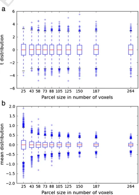
796 An important question is whether the counting statistic introduced in 797 Eq.(1)is a valid statistic to detect activated voxels. One essential criteri-798 on for this is to check the pivotality, i.e. the convergence–under the null 799 hypothesis–of the statistic distribution toward a law that is invariant 800 under data distribution parameters. In the present case, the main devia-801 tion from pivotality could result from a distribution of (extreme) statis-802 tical values that depends on the parcel size: large parcels would 803 represent fMRI signal averaged over larger domains, and thus would 804 get typically lower values. This is indeed typically the case for the 805 mean statistic (seeFig. B.12(b)); however, we show for instance that 806 the t statistic used in“Materials and methods”is very weakly influenced 807 by the parcel size: we repeated the experiment described in“Materials 808 and methods”, i.e. computing the t statistic on parcels obtained by 809 Ward's algorithm, based on 100 random batches of 20 subjects, after per-810 mutation by random sign swap. We tabulate the t distribution according 811 to the parcel size by using 10 size bins. The result, shown inFig. B.12(a), 812 is that the effect, if any, is not detectable by visual inspection.
813 To test more precisely the independence on the t distribution with 814 respect to the parcel size, we tested the equality of the mean, median 815 and variance of the size-specific distributions using the One-way 816 (mean), Kruskal (median), Bartlett (variance), Levene (variance) and 817 Fligner (variance) tests as implemented in the SciPy library.5 All 818 the tests are performed on the 10 bins jointly. We obtain the following 819 p-values: One-way,P= 0.36; Kruskal,P= 0.27; Bartlett:P= 0.95;
820 Levene:P= 0.016; Fligner:P= 0.06. This means that there is only a
821 small effect on the variance, as reported by the Levene test, that is
822 more sensitive than Fligner (which is non-parametric) and Bartlett,
823 which assumes Gaussian distributions. However this effect is very
824 small, and has no obvious consequence on the number of peak values
825 of the statistic; in particular, we do not observe monotonic trends
826 with size. Note that the small effect fades out when using larger number
827 of subjects (here, onlyn= 20 subjects per groups were used). Finally,
828 we did notfind any significant correlation between the number of
de-829 tections above a given threshold (using uncorrected p-values of 10−2,
830 10−3, 10−4) and the parcel size.
831 In conclusion, the effect of parcel size is too small to jeopardize the
832 usefulness of the counting statistic.
[image:12.595.91.501.58.196.2]z = _10
[image:12.595.62.296.230.398.2]Fig. A.10.Example parcellations obtained with Ward's clustering algorithm. The [angry faces–control] fMRI contrast maps of 20 bootstrapped subjects were used.
Fig. A.11.Size and compactness of the parcels obtained with Ward's clustering algorithm on fMRI contrast maps. For each parcel, the compactness is measured as the difference between a mask of the parcel and its 1-eroded image). One can observe a great variability in parcel size/compactness, which reflects the structure of the individual fMRI contrast maps.
Fig. B.12.Impact of the parcel size on the distribution of the second-level one-sample t sta-tistic (a) and of the mean value (b). While there is an obvious effect on the mean, there is no conspicuous effect on the t distribution.
5
[image:12.595.306.550.373.713.2]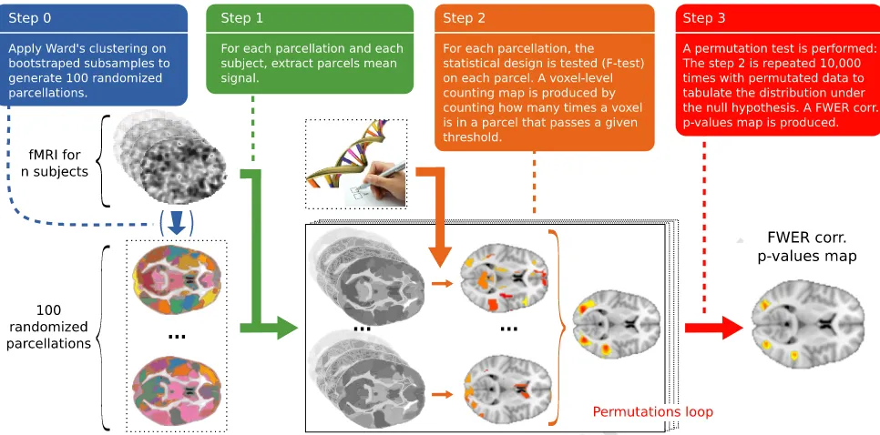


![Fig. 6. Negative logp-value associated with a non-zero intercept test with confounds (handedness, site, sex), on a [angry faces–control] fMRI contrast from the faces protocol](https://thumb-us.123doks.com/thumbv2/123dok_us/1509745.692514/8.595.50.535.227.710/negative-associated-intercept-confounds-handedness-control-contrast-protocol.webp)