A Novel Decoder Based on Parallel Genetic Algorithms for
Linear Block Codes
Abdeslam Ahmadi1, Faissal El Bouanani2, Hussain Ben-Azza1, Youssef Benghabrit1 1Department of Industrial and Production Engineering, Moulay Ismail University,
National High School of Arts and Trades, Meknès, Morocco
2Department of Communication Networks, National High School of Comptuer Science and System Analysis, Rabat, Morocco
Email: [email protected], [email protected], [email protected], [email protected]
Received November 8, 2012; revised December 5, 2012; accepted December 15, 2012
ABSTRACT
Genetic algorithms offer very good performances for solving large optimization problems, especially in the domain of error-correcting codes. However, they have a major drawback related to the time complexity and memory occupation when running on a uniprocessor computer. This paper proposes a parallel decoder for linear block codes, using parallel genetic algorithms (PGA). The good performance and time complexity are confirmed by theoretical study and by simu- lations on BCH(63,30,14) codes over both AWGN and flat Rayleigh fading channels. The simulation results show that the coding gain between parallel and single genetic algorithm is about 0.7 dBat BER = 10−5 with only 4 processors.
Keywords: Channel Coding; Linear Block Codes; Meta-Heuristics; Parallel Genetic Algorithms; Parallel Decoding Algorithms; Time Complexity; Flat Fading Channel; AWGN
1. Introduction
The error correcting codes began with the introduction of Hamming codes [1] in the same period that the remark- able work of Shannon [2]. They consist in correcting data corruption when saved in storage media (erasure CD/ DVD, etc.) or transmitted over noisy communication channel. Figure 1 shows the canonical system diagram of numerical communication.
The encoder takes the information symbols and adds to them redundancy symbols, carefully chosen such that a maximum of errors, which are infiltrated throughout the process of signal modulation, noisy transmission channel, and demodulation, can be corrected. The result- ing binary code word is then transmitted over the noisy and memoryless channel under assumption that the sending messages are independent from the added noise. At the reception, the decoder attempts, given channel observations and using the redundancy symbols, to find the most probable message. The techniques used by the decoder are diverse. The most optimal criterion is Maxi- mum Likelihood [3]. Given its high complexity (compu- tation time, memory occupation), other suboptimal tech- niques with acceptable performance are used in practice like Turbo codes [4] and LDPC [5]. Several other decod- ers developed were inspired from the artificial intelli- gence field as Han decoding which using algorithm A* [6], Genetic Algorithms (GAs) [7] and Neural Networks
[8]. In 2007, it was shown that decoders based on GAs have good performance and time complexity lower than those of classical algebraic decoders [9]. In 2008, the performance of these decoders has been further improved by using iterative decoding for product block codes in two dimensions [10]. In 2012, we made an extension of concatenated codes by passing to three dimensions [11]. In this last work, we have proposed two iterative decod- ing algorithms based on GAs, which can be applied to any arbitrary 3D binary product block codes, without the need of a Hard-In Hard-Out decoder.
The first decoder outperforms the Chase-Pyndiah [12] one. The second algorithm, which uses the List-Based
SISO Decoding Algorithm (LBDA) based on order-i re- processing [13], is more efficient than the first one. We have also showed that the two proposed decoders are less complex than both Chase-Pyndiah algorithm for codes with large correction capacity, and LBDA for large i pa- rameter.
Modulation
Information
Source Encoder
û
v
u 1 11 1
1
n
k k kn
b b b
G
b b b
x r Demodulation Destination Decoder Noisy Channel y
0,1
2 n
1 , 2 .
n x xn
2
2and . Figure 1. The canonical diagram of numerical communica- tion.
we have developed a new decoder using parallel genetic algorithms, which runs on a parallel computer with mul- tiple processors and a shared memory, or on a distributed system. So, it reduces the time complexity and increases little performance.
This paper is organized as follows. Section 2 presents some background on Linear Block Codes, Parallel Sys- tem, and Genetic Algorithms. Section 3 describes the pro- posed Parallel Genetic Algorithms Decoder (PGAD), studies its time complexity and compares it with the one of SGAD. In Section 4 we discuss the simulation results obtained for PGAD. Finally, we give in Section 5 our conclusions and perspectives of this work.
2. Background
2.1. Linear Block Codes
Let 2 be the binary alphabet and The set of all words of length ni.e.:
2 1 / ,n
x x
A linear code C of length n on is a subspace of the vector space
n [14]. i.e.:2
, , , ,
x y C x y C x C
,
Let x y C such that x
x1, , xn
1, , nand
y y
,H
d x y
yi,1 i n
.
x y, /xy
dim
k C
y . The Hamming distance between x and y, noted , is defined by:
, card /H i
d x y i x
The minimum Hamming distance d of a code C is the Smallest non zero distance between all its vectors, taken two by two. i.e.:
, min H x y C
d d
(1)
Let be the dimension of code C. C is then said d n k d, ,
-linear code. The code rate is the ratiok n
Let
Thus, we have:
/ 2
k
C G
1 ,
n
x
i.e. x C
x
1
2! , ,k k
such that xG
1 1 11 1
1 1
k k
n n k kn
x b b
i.e:
1, , k
be a basis of C. Since iB b b b C,
Then length (bi) = n. The matrix G for which rows are the basis vectors is called generating matrix of the code
C. It can be written as:
x b b
2.2. Parallel Systems
The choice of parallel machines or distributed systems is more imposed for applications requiring a very high processing power and/or a big memory space. There are plenty of parallel systems which are classified as below [15].
2.2.1. Taxonomy of Parallel Systems
These systems have been classified by Flynn (1972) ac- cording to two independent concepts: the stream of in- structions and the stream of data used by these instruc- tions. There are four possible combinations:
SISD (Single Instruction, Single Data): The machine executes one instruction on one data at each clock cy- cle. It is not really a parallel machine but a classical computer (Von Newman).
SIMD (Single Instruction Multiple Data): A processor having a single Control Unit (CU) and multiple Ar- ithmetical and Logical Units (ALUs) executes the same instruction on different data at each clock cycle.
MISD (Multiple Instruction, Single Data): Systems running multiple instructions on the same data at each clock cycle.
MIMD (Multiple Instruction Multiple Data): These systems are multiple independent processors i.e. each processor has its CU and its ALU. At the same clock cycle, each processor executes a different instruction on a different data. These instructions can be synchro- nous or asynchronous. The majority of parallel sys-tems are MIMD. The MIMD system can be either a Multiprocessor or a Multi-computer or a hybrid of them. We explain in the next subsections the architec- ture of each one.
2.2.2. Multiprocessor
memory which composed of several memory blocks Figure 2. These blocks are interconnected with the pro- cessor and between them [15].
If two processors want to communicate, it suffices that the first one writes data (or message) in the memory and the other one recuperates it. So their programming is easy since the programmer does not have to focus on the explicit communication (message exchange) between the different processors. These allowed multiprocessors mak- ing a great success. However, it would be difficult to build a multiprocessor when the number of its commu- nicating elements (processors and memory blocks) is very important. Indeed, the interconnection of all these elements is not always an easy task.
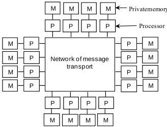
2.2.3. Multi-Computer
[image:3.595.337.501.218.343.2]A multi-computer is also a MIMD system but relatively simple to build. It contains a number of computers (CU + ALU + private memory) linked together by an intercon- nection network. Each computer has its own memory Figure 3. This reduces significantly the number of ele- ments to be interconnected. The communication between computers is achieved by exchanging messages as primi- tives Send/Receive, programmed and integrated by the programmer in its application [15]. This may complicate more his task. The following points must be taken into account for each parallel programming:
For an efficient communication between different elements (processors and memory blocks) of a paral- lel or distributed system, the suitable choice of the topology, routing and switching mode of its inter- connection network affects its performance remarka- bly.
To benefit from the advantages of a multiprocessor and those of a multi-computer and minimize the dis- advantages of each one of them, hybrid systems have been designed.
To take advantage of parallel systems, we must exe- cute on them parallel programs or containing a sig- nificant part of parallel instructions.
2.3. Genetic Algorithms
The Genetic Algorithm (GA), initiated in 1970 by Hol- land [16] is an Evolutionary Algorithm (EA) inspired from the natural biological evolution. It use search sto- chastic techniques to solve problems not having an ana- lytical resolution or when the time to resolve them by classical algorithms is not reasonable [17]. Their applica- tions cover, in addition to error correcting codes in tele- communication, several other fields as optimization, arti- ficial intelligence, economic markets, etc. As shown in algorithm below [18], an EA especially a GA has an it- erative character:
Sharedmemory
P P P P
P
P P Processor
P
P P P P
P P
P P
Figure 2. A multiprocessor with 16 processors sharing a commonmemory.
Processor
Network of message transport
P P P P
P
P P
P
P P P P P
P P P
M M M M
M M M M M
M M
M Privatememory
M M M M
Figure 3. A multi-computer with 16 interconnected proces-sors where each one has its own memory.
t=0;
initialize and evaluate [P(t)]; while not stop-condition do
P’(t)=variation [P(t)];
Evaluate [P’(t)];
P(t+1) =select [P’(t), P(t)];
t=t+1; end while.
PIt generates an intermediate population t by ap- plying variation operators (often stochastic) on individu- als (which may be here, information sequences or code- words) of the current population P(t). Then, it evaluates the quality (of being solution) of individuals from P t
using a criterion known as fitness. It finally creates the new population P(t+1) in which individuals are selected from those of P t
and eventually from P(t). The pro- cess is repeated until the stopping condition is satisfied. In general, the process is stopped when the optimal solu-tion is found or when the maximum number of itera- tions is reached.The Genetic Algorithms can be singles (SGA) or Par- allels (PGA).
2.3.1. Single Genetic Algorithms
The previous general algorithm can be adapted in SGA as follows:
Generate an initial population of n individuals randomly; while not stop-condition do
while not Filled-New-Population do
Select two parent individuals;
Cross them to have a new(s) individual(s);
The new individuals undergo eventual mutations;
Insert the new individual in the new population; end while
Replace the old population by the new one; end while.
The three classical operators inspired from natural evolution to generate a new population from the current one in both SGA and PGA are selection, crossover and mutation:
The selection operator describes how to select the parents in the current population to cross them and generate new individuals (offspring) which will be inserted in the new population. The individuals are sorted in ascending order of their fitness to give more chances to the best ones (fittest) to be selected (as- suming that better parents reproduce better children). However, there are cases where the crossing of bad parents can generate good offspring. The most popu- lar selection methods are: Proportional, Linear Rank- ing, Whitley’s Linear Ranking and Uniform Ranking [19].
The crossover operator generates new individuals inheriting from their parents. i.e. Their genes are a mixture of those of their parents. There are several crossing techniques that can be either generic (robust)
i.e. applied in a wide variety of problems, or specific to particular problems, or hybrid techniques combin- ing generic and specific ones.
As in natural evolution, the genes of some individuals may undergo changes (mutations). This occurs in very rare cases. The mutation plays a very important role in the convergence of SGA and PGA algorithms. Indeed, it will prevent their premature convergence by guid-ing them to explore other more promisguid-ing areas and avoid a local optimum.
2.3.2. Parallel Genetic Algorithms
The PGAs are GAs running on parallel systems dis-cussed in the second subsection.Their purpose is not only accelerating the convergence and/or use a large memory space but also improve the performance. There are two models of PGAs: 1) Island model (or network model) which runs an independent GA with a sub-population on each processor, and the best individuals are communi-cated either to all other sub-populations or to neighboring population [20]; 2) Cellular model (or neighborhood model) which runs an individual on each processor, and cross with the best individual among its neighbors [21]. In fact, the second model is a particular case of the first one. Indeed, its population is reduced to a single indi-vidual on each processor.
The general algorithm of PGAs is given below:
Generate an initial population of n individuals randomly; while not stop-condition do
Calculate the fitness f (x) for any individual x; if Interval-Exchange then
Exchange of individuals; end if
while not Filled-New-Population do
Select individual parents;
Cross them to make new people;
New individuals undergo eventual mutations;
Insert new individuals in the new population; end while.
Replace the old population by the new one; end while.
3. The Proposed Parallel Decoder Based on
Genetic Algorithms
This work is a parallelization of the decoder that we have already used in [9,10], and [11] by exploiting some tech- niques of parallel genetic algorithms used in other do- mains like Optimization and Artificial Intelligence. It can be run on a multiprocessor where the data exchanged are saved in global or shared variables, or on a multi-com- puter which exchange data between its processors via a network.
1 n
Let F F, , F and
1 n
be respec- tively the fading vector and the received sequence (asso- ciated to the transmitted sequence) at the decoder input of a binary linear block code C(n,k,d) with a generator matrix G. The parameters Np, Ne, Nc, Nm, Ns, Ng are re- spectively the population size, elite number, offspring number, migrant number, processor number and maxi- mum number of generations such that, ,
R R R
1
m p e c s
N N N N N
1
1 πR R
is a positive integer.
3.1. The PGAD Algorithm
The sub-algorithm which will run in parallel on each pro- cessor is given below:
Step 0:Initialization
Sort the elements of the received vector R in de-scending order of their magnitude to produce another vector R(1) i.e. find a permutation π1 such that
and 1 1 1
1 2 n
R R R
1
. This will put reliable elements in the first ranks. F is the
permutation of F by π1 i.e. 1
1
πF F
π
. Then,
permute G by 2 to produce G′ such that the first k
columns of G′ are linearly independent i.e.
π
G G 1
R 1
2 . The two vectors and F are
permuted by π2 to R and F.
So,
1
2 2 1
π π π π
12 2
π π
π1
π
F F F F
π π π
, with
2 1
Quantize the first k bits of R to obtain binary vec-tor r and randomly generate Np −1 information vec-tors of k bits each one. These vecvec-tors form with vector r the initial population of Np individuals
1, ,
.
Np
I I ;
1:Reprod
Step on
ent generation number).
of the current population, using
n
dis-
, i 1, , Np
Sort the current population individuals in descending
iduals (elites) from the current
− Ne individuals of the
ty pc the selected parents to
gen-ls with a probability pm if
duals with their fitness in
ucti
gen←0 (gen is the curr
While(gen < Ng)do
Encode individuals
G′ to obtain code words: Ci = IiG′(1 ≤ i ≤ Np);
Compute individual fitness, defined as Euclidia tance between Ci and R:
n
2f C
C R1
i ij j
j
order of their fitness;
Copy the Ne best indiv population to the new one;
Select parents from the Np current population;
Cross with probabili erate Nc new individuals;
Mutate the new individua their parents are crossed;
Insert these Nc new indivi the new population Figure 4;
Send the best
Nc N 1 indi-new
m the
ecision
1m
N NpNe
ir fitness) to the s
viduals (with the populations of
Ns −1 other processors as shown in Figure 5;
Receive Nm migrant elites (with their fitness) fro previous population of each Ns −1 other processors,
to complete the new population as shown in Figure 6;
Replace the current population with the new one;
gen←gen+1;
end while Step 2: D
Get the best individuals
s
i
i N
D
of last popula-
tions of all processors. The best one D′ of them is the closest to R′. i.e. D argmin
D i R ,1 i Ns
.
1 π
D D . So, the decided codeword is
. . . . .
. .
Nm elites
[image:5.595.354.494.86.216.2]. . . . . . . Current population New population
Figure 4. The ith processor which works on the current population to give the next one.
. . . . . . . . . . . . . .
Neelites
Ncchildre
n
Nm elites
Nm elites
. . . . . . . . . . . . . .
Neelites
Ncchildre
n . . . . . . . . . . . . . .
Ne elites
Nc children
. . . . . . . . . . . . . .
Ne elites
[image:5.595.347.499.255.397.2]Nc children … …..
Figure 5. In a given generation, the ith processor sends its best N individuals to other processors.
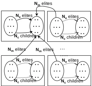
Nm elites Nm elites
m
Nm elites
. . . . . . . . . . . . . .
Ne elites
Nc children
. . . . . . . . . . . . . .
Ne elites
Nc children
. . . . . . . . . . . . . .
Ne elites
Nc children
. . . . . . . . . . . . . .
Ne elites
Nc children
… …..
Figure 6. In a given generation, the ith process eceives the best N individuals from each other processor
ustrated
haracteristics
PGA are [19]:
of the evolution step in a
ucing Operators
1
e NeNc in the new
like in our wor or r
. m
The flowchart of the previous algorithm is ill inFigures 7 and 8.
3.2. The PGAD C
The main elements characterizing a basic
evolution mode, reproduction operators (crossover and mutation), selection and replacement policy of individu-als (local and foreign) and migration.
3.2.1. Evolution Mode It defines the granularity
sub-algorithm of the PGA. i.e. how the new population is created from the current one. There are two techniques that are often used. The first one is the generational GA (GGA) where the new population replaces all the old ones. The second technique inserts only a few new (gen-erated) individuals in the current population. In our im-plementation, we have used the GGA evolution mode with elitism.
3.2.2. Reprod
To generate Nc individuals
Ii N i [image:5.595.57.289.563.707.2](1)best indiv.
( −1) best indiv.
Loop
Initialization step
To the new populations of
Ns-1 other
processors Crossing the selected parents and mutating the children
Coding and fitness computing
Forming the new population
Sorting fitness gen gen+1
gen =Ng
Nc new
individuals
Ne first
individuals
Ne +Nc individuals
Np
individuals
No
Yes
Np sorted
individuals
…. ….
Nm best
individuals Nindividuals m best
Np - Ne
[image:6.595.59.287.77.498.2] [image:6.595.61.284.543.591.2]individuals
... ...
From previous populations of Ns-1
other processors
Np sorted
individuals
R’
R,F,G
Np sorted
individuals Descending
sort of the magnitudes
and permutations
Adding r
to Np-1
individuals of k bits randomly generated
Coding wit
G’, fitn computing, and sorting of the Np
individuals F’,G’ h ess Np individuals Quantizing of the first k bits r
′ ( )= ′ 1 ( )
= ′1( )
← 0
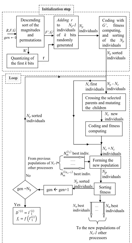
Figure 7. The flowchart of the proposed PGAD sub-algo- rithm running on the ith processor.
Figure 8. The codeword decision flowchart of the proposed PGADalgorithm.
o individuals as parents ( , ) using the following linear ranking:
Selection of tw P Q
max max
weight 2 1 weight 1
weighti i
N
,
1 1, , .
p p i N (2)
where weighti is the ith individual weight and weightmax is the weight assigned to the fittest (closest) individual.
- Let pc, pm be respectively, the probabilities of cross-over and mutation, and let Rand be a uniformly ran dom value between 0 and 1, generated at each time.
if Rand < pc then
1, ,N N
,j
1, ,k
: i Ne e c
0
4
if Rand 1
1 e else
j
j j
j
j j j j R F
N ij
j
P Q
P P P Q
I Q (3) and then
1 ij if Rand m
Iij I p
if Rand 0.5 else P Q end if.
We note that on an AWGN (Additive White Gaussian hannel) channel, we have
else
i
I
Noise C
1, 1, ,
j
F j k .
3.2.3. Selection and Replacement Str gies
They define the selection of individuals to replace in the d those to
more
domly. In
This is an operation that helps to diversify and enrich the a sub-algorithm which runs in a pro-
ate
current population of a sub-algorithm PGA an
migrate from other processors. The individuals can be replaced by new local ones or by the migrant ones:
The main replacement policies are [19]: 1) Inverse Proportional; where the worst individual is likely to be replaced; 2) Uniform Random; where all individuals have the same chance of being replaced; 3)
Worst; where the worst individual is always re- placed. In some problems, it is replaced only if it is worse than the new one; 4) Generational; where the entire current population is replaced by a new one. In our work, we keep the best local individuals (elitism) and the bad ones are replaced by new local offspring and by the migrants from other processors.
There are two cases to choose migrant individuals: choose the best ones, or choose them ran
our algorithm, we chose the best migrants.
3.2.4. Migration
new population of
The exchange (send/receive) of individuals is done in two modes: synchronous or asynchronous.
The synchronous mode suspends, periodically, the execution of a sub-algorithm of the PGA and waits for th
e receiving migrant individuals from other nodes be- fore continuing its execution. In asynchronous mode, the sub-algorithm does not wait. Once the migrant individu- als arrive, it deals with them.
In our algorithm, we send/receive at each new popula- tion the
N 1 first best indi-duce the num
ty
A PGA is called homogeneous if its nodes run the same erwise, it is called heterogeneous.
of the different stages m PGAD in the
e almost always, ability is close to 1. So its time com
ion will occur rarely since its pro-
T e PGAD.
m p e c
N N N N s
ualsto/from every other processor according to the
asynchron ber of messages
that flow through the network connecting processors, the number of migrant individuals should be less than the number of individuals locally generated for each new population. i.e. NmNeNc.
3.2.5. Heterogenei vid
ous mode. To re
type of algorithm. Oth
Our PGAD is homogeneous. Indeed, all nodes are sym-metric and perform the same genetic algorithm having same parameters and operators.
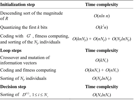
3.3. PGAD Time Complexity
We give in Table 1 the complexity
of the proposed decoding algorith order
-oftheir appearance in the flowcharts of Figures 7 and 8 before deducting its global complexity.
We note that:
The crossover operation will be mad since its prob
plexity is O(kNc).
The complexity of mutation operation is neglected. Indeed, this operat
bability is close to 0.
The total time complexity of PGAD is then:
able 1. Time complexities of different steps of th
Initialization step Time complexity
Descending sort of the magnitude
of R O(nln n)
Quantizing the first k bits
Coding with
O(k2n)
G, fitness computing,
duals O(knNp) + O O(NplnNp)
vectors
g O(knN nNc)
uals O p p)
and sorting of the Np indivi
(nNp) +
Loop steps
Crossover and mutation of
Time complexity
information O(kNc)
Coding and fitness computin Sorting of Np individ
c) + O(
(N lnN
Decision step Time complexity
Sorting of i, 1 s
D i N O(NslnNs)
2
2
1 ln n
ln
ln ln
p p p
lln ln p
g c c c p p s s
p g c
g p p s s
k n knN nN N
N kn nN N N N
O n n k n kn N N N
N N N N N
(4)
From the formula (4), it is clear that the complexity of PGAD is lower than that of SGAD. Indeed, there are te
essors (Ns = 4). To study the d PGAD decoder, we have
lation Size
de-
O n n N
N k N
N
rms that are common to both decoders (initialization and sorting at the end of the loop). The term NslnNs can be neglected when the processor number is small. The difference between SGAD and PGAD consists in the crossing, coding, and fitness computing in the loop. For each generation, we must cross parents to have Np ‒Ne
new individuals in the case of SGAD against only Nc in PGAD (Nc< Np‒Ne). Likewise we encode in the loop only Nc individuals in our decoder against Np ‒ Ne in SGAD. For the fitness in the loop, it is also computed for
Nc individuals instead of Np‒Ne.
From the foregoing, we can summarize the advantages of our decoder as follows:
Improvement of performance. Indeed, It corrects er-rors better than simple algorithms studied in [9,10] as shown in simulation section.
Reducing the time complexity of the decoding pro- cess: 1)It is run in parallel on multiple processors for almost the same number or lower of total individuals (NgNp) used in a single decoder; 2)It reduces the time of encoding and fitness computing, since the algo- rithm receives (Np − Ne − Nc) migrant individuals (encoded) with their fitness already computed; 3) It reduces the reproduction time since the number of parents to cross is reduced to Nc(Nc < Np − Ne).
4. Simulation Results
Our PGAD is run on 4 proc performance of the presentesimulated a binary communication system with BPSK modulation and both AWGN and Rayleigh fading chan- nels. We give in this section, the impact of each parame- ter Ng, Np, pc, pm, Ne, Nc and code rate on the performance of our decoder and we finish with a comparison with the SGAD decoder. The chosen code is the linear block
BCH(63,30,14) code. The minimum number of sent er- roneous frames is 30. The performance will be given as figures showing the Bit Error Rate (BER) versus the en- ergy per bit to noise power spectral density ratio Eb/N0.
The figures corresponding to each channel are given in Table 2.
4.1. Effect of Generation Number and Popu
[image:7.595.57.288.563.737.2]Table 2. Simulation figures corresponding to each channel.
AWGN channel Fading channel
Figures 1 to 14 Figure 15
words N ability to find the codeword closest the in becomes high. T
ossi-The crossover is a very important operation insofar as it an effective exploitation.
The effect of mutation rate for BCH(63,30,14) is de- n that pm = 0.03 is the op-
Among the best individuals of the current population, new population. This
pNg, the prob put sequence
to his makes it p
ble to improve the BER performances. The effect of in-creasing the number of evaluated code words on the BER
improvement for code BCH(63,30,14) at the 12th itera-tion is presented in Figures 9 and 10. The values Ng = 100 and Np = 100 can be the optimal values in a large range Eb/N0. The other genetic parameters for the first optimization are: Np = 100, Nc = 80, Ne = 5, pc = 0.99, pm = 0.03 and Ng = 100, Nc = 80, pc = 0.99, pm = 0.03 for the second one.
[image:8.595.319.529.87.250.2]4.2. Crossover Rate Effect
Figure 9. Effect of the generation number for BCH(63,30,14).
allows a large exploration, and
In Indeed, it creates new individuals may be good solu- tions to the problem. For most problems, the probability of crossover is high. This is the case also for the error correcting. The Figure 11 shows that among the studied probabilities pc= 0.99 offers the best performance. For this simulation, we have fixed the other parameters as follows: Ng = 10, Np = 100, Nc = 80, Ne = 5, and pm = 0.03.
4.3. Mutation Rate Effect
Figure 10. Effect of the population size for BCH(63,30,14). picted in Figure 12. It is show
timal BER value for all SNRs. One reason of this value close to 0 may be the stability of members in vicinity of optima for low mutation rates. The fixed values are: Ng = 100, Np = 100, Nc = 80, Ne = 5, and pc = 0.99.
4.4. Elite Number Effect
some may survive and move to the
can be justified by the fact that their elitism may give birth to other best descendants. As shown in the Figure 13, the greater the number of elites survived, more per- formances improve. However, when we exceed five el- ites the performances begin to decline. We deduce that worse individuals can also create, by crossover and mu- tation, better individuals. So we choose Ne = 5. The fixed values for this simulation are: Ng = 100, Np = 100, Nc = 80, pc = 0.99 and pm = 0.03.
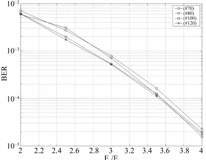
4.5. Offspring Number and Migration Rate Effects
Figure 11. Effect of the crossover probability for BCH(63,30,14).
The number of individuals migrating from each nodeis
NpNeNc
Ns 1
9Nc
3.So when er decreases, tthis num- he number of individuals created locally
c increases. From the curves plotted formances increase when Nc increases b
N in Figure 14,
[image:8.595.320.530.283.448.2] [image:8.595.320.526.481.645.2]Figure 12. Effect of the mutation rate for BCH(63,30,14).
Figure 13. Effect of the elite number for BCH(63,30,14).
Figure 14. Effect of the offspring number for BCH(63,30,14).
Nc = 80. We also note that when there is no ex- change of
ls is equal to 0) the performance is worse than with the
51). From the when the rate decreases, per- is explained by the fact that
ance of our PGAD on a n- 3. We and 17 that the parallel
applied to any linear block ions show that it provides better per- ecoder based on SGA and the gain is
individuals (Nc = 95 i.e. the number of migrant individu-a
exchange. The fixed values of parameters are: Ng = 100,
Np = 100, Ne = 5, pc = 0.99 and pm = 0.03.
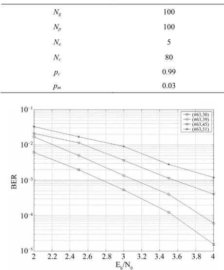
4.6. Code Rate Effect
We have studied the performance of the following BCH codes: (63,30), (63,39), (63,45), and (63,
Figure 15, we note that formance increases. This
when the code length n increases for the same dimension
k;the number of redundancy bits (check) increases. i.e. it corrects better with more redundancy; which makes sense. In this simulation, we adopted the optimal values in Table 3 previously found.
4.7. Performance Comparison between PGAD and SGAD
We have studied the perform
Gaussian channel AWGN and flat Rayleigh fading cha nel with flat fading using the same parameters in Table
remark from Figures 16
coder not only reduces the time complexity, but also has good performance compared to simple decoder studied in [9] and just for 4 processors.
5. Conclusion
We have presented a new decoder based on parallel ge- netic algorithms which can be
code. The simulat formance than a d
Table 3. Time complexities of different steps of the PGAD.
Ng 100
Np 100
0
Ne 5
Nc 80
pc 0.99
pm .03
[image:9.595.67.278.481.645.2]Figure 16. Pe n SGAD and PGAD on AWGN channel for BCH(63,30,14).
rformance comparison betwee
Figure 17. Performance comparison between SGAD and PGAD on Rayleigh channel for BCH(63,30,14).
about 0.7 dBwith 4 processors only. This is due to its parallel architecture which can exploit and explore more individuals and avoid the premature convergence to optimum. In addition, this decoder has a lower com ity because it runs on multiple processors simultaneously and because it reduces the time of encoding and fitness computing, and the time of generation of new individuals. Its performance can be further improved by adju algorithm parameters and characteristics (processor num- ber, topology, migration, selection and replacement, ...) and by parallelizing tasks running on the same processor or by putting it in hybrid with other decoders. We could also envisage an iterative decoding based on PGAs.
local plex- ,
sting
,
REFERENCES
[1] R. W. Hamming, “Error Detecting and Error Correcting Codes,” Bell System Technical Journal, Vol. 29, No. 2, 1950, pp. 47-160.
[2] C. E. Shannon, “A Mathematical Theory of
Communica-tion,” Bell System Technical Journal, Vol. 27, 1948, pp. 379-423, 623-656.
[3] S. Roman, “Introduction to Coding and Information The-ory,” Spring Verlag, New York, 1996.
[4] C. Berrou and A. Glavieux, “Near Optimum Error Cor-recting Coding and Decoding: Turbo Codes,” IEEE Trans- actions on Communications, Vol. 44, No. 10, 1996, pp. 1261-1271. doi:10.1109/26.539767
[5] D. J. C. Mackay and R. M. Neal, “Good Codes Based on Very Sparse Matrices,” 5th IMA Conference on Cry raphy and Coding, Lecture Notes in Computer Science
ptog-number 1025, Oc 00-111.
doi:10.1007/3-tober 1995, Springer, Berlin, pp. 1 540-60693-9_13
[6] Y. S. Han, C. R. P. Hartmann and C.-C. Chen, “Efficient Maximum Likelihood Soft-Decision Decoding of Linear Block Codes Using Algorithm A*,” Technical Report
s for Soft Decision Decoding of Lin-SU-CIS-91-42, Syracuse University, Syracuse, 1991. [7] H. S. Maini, K. G. Mehrotra, C. Mohan and S. Ranka,
“Genetic Algorithm
ear Block Codes,” Journal of Evolutionary Computation, Vol. 2, No. 2, 1994, pp. 145-164.
doi:10.1162/evco.1994.2.2.145
[8] J. L. Wu, Y. H. Tseng and Y. M. Huang, “Neural Net-works Decoders for Linear Block Codes,” International Journal of Computational Engineering Science, Vol. 3, No. 3, 2002, pp. 235-255.
doi:10.1142/S1465876302000629
[9] F. El Bouanani, H. Berbia, M. Belkasmi and H. Ben-Azza, “Comparison between the Decoders of Chase, OSD and Those Based on Genetic Algorithms,” 21 Colloquium of GRETSI (Group of Study and Signal and Pictures Pro- cessing), Troyes, 11-14 September 2007, pp. 1153-1156. [10] M. Belkasmi, H. Berbia and F. El Bouanani, “Iterative
Decoding of Product Block Codes Based on the Genetic Algorithms,” 7th International ITG Conference on Source and Channel Coding (SCC’08), Ulm, 14-16 January 2008, pp. 1-6.
[11] A. Ahmadi, F. El Bouanani, H. Ben-Azza and Y. Beng- habrit, “Reduced Complexity Iterative Decoding of 3D-
odes,” IEEE Proceed-Product Block Codes Based on Genetic Algorithms,” Jour- nal of Electrical and Computer Engineering, Vol. 2012, 2012, Article ID: 609650.
[12] R. Pyndiah, A. Glavieux, A. Picart and S. Jacq, “Near Optimum Decoding of Product C
ings of Global Telecommunications Conference, San Fran- cisco, 28 November-2 December 1994, Vol. 1, pp. 339- 343.
[13] P. A. Martin, D. P. Taylor and M. P. C. Fossorier, “Soft- Input Soft-Output List-Based Decoding Algorithm,” IEEE Transactions on Communications, Vol. 52, No. 2, 2004, pp. 252-264.
[14] S. Lin and D. Costello, “Error Control Coding: Funda-mentals and Applications,” Prentice-Hall, Upper Saddle River, 1983.
[15] A. Tanenbaum, “Computer Architecture,” Dunod, Paris, 2001.
[image:10.595.65.280.294.463.2]Sys-Algorithms in Search,
Optimi-on, Vol. 6, No. 5, 2002, pp. 443-462.
tems,” University of Michigan Press, Ann Arbor, 1975. [17] D. E. Goldberg, “Genetic
zation, and Machine Learning,” Addison-Wesley, Boston, 1989.
[18] E. Alba and M. Tomassini, “Parallelism and Evolutionary Algorithms,” IEEE Transactions on Evolutionary Com-putati
[19] E. Alba and J. M. Troya. “A Survey of Parallel Distrib-uted Genetic Algorithms,” Complexity, Vol. 4, No. 4, 1999, pp. 31-52.
doi:10.1002/(SICI)1099-0526(199903/04)4:4<31::AID-C PLX5>3.0.CO;2-4
[20] T. Starkweather, D. Whitley and K. Mathias, “Optimiza-tion Using Distributed Genetic Algorithm,” Springer Verlag, New York, 1991, pp. 176-185.
doi:10.1007/BFb0029750
[21] V. S. Gordon and D. Whitley, “A Machine-Independent Analysis of Parall
tems, Vol. 8, 1994, pp. 181-214.