LIMSI Submission for WMT’14 QE Task

LIMSI Submission for WMT’14 QE Task

Guillaume Wisniewski and Nicolas P´echeux and Alexandre Allauzen and Franc¸ois Yvon Universit´e Paris Sud and LIMSI-CNRS

91 403 ORSAY CEDEX, France

{wisniews, pecheux, allauzen, yvon}@limsi.fr

Abstract

This paper describes LIMSI participation to the WMT’14 Shared Task on Qual-ity Estimation; we took part to the word-level quality estimation task for English to Spanish translations. Our system re-lies on a random forest classifier, an en-semble method that has been shown to be very competitive for this kind of task, when only a few dense and continuous fea-tures are used. Notably, only16 features are used in our experiments. These fea-tures describe, on the one hand, the qual-ity of the association between the source sentence and each target word and, on the other hand, the fluency of the hypothe-sis. Since the evaluation criterion is the f1 measure, a specific tuning strategy is

proposed to select the optimal values for the hyper-parameters. Overall, our system achieves a 0.67 f1score on a randomly

ex-tracted test set. 1 Introduction

This paper describes LIMSI submission to the WMT’14 Shared Task on Quality Estimation. We participated in the word-level quality estimation task (Task 2) for the English to Spanish direction. This task consists in predicting, for each word in a translation hypothesis, whether this word should be post-edited or should rather be kept unchanged. Predicting translation quality at the word level raises several interesting challenges. First, this is a (relatively) new task and the best way to for-mulate and evaluate it has still to be established. Second, as most works on quality estimation have only considered prediction at the sentence level, it is not clear yet which features are really effective to predict quality at the word and a set of base-line features has still to be found. Finally, sev-eral characteristic of the task (the limited number

of training examples, the unbalanced classes, etc.) makes the use of ‘traditional’ machine learning al-gorithms difficult. This papers describes how we addressed this different issues for our participation to the WMT’14 Shared Task.

The rest of this paper is organized as follows. Section 2 gives an overview of the shared task data that will justify some of the design decisions we made. Section 3 describes the different features we have considered and Section 4, the learning methods used to estimate the classifiers parame-ters. Finally the results of our models are pre-sented and analyzed in Section 5.

2 World-Level Quality Estimation

WMT’14 shared task on quality estimation num-ber 2 consists in predicting, for each word of a translation hypothesis, whether this word should be post-edited (denoted by the BAD label) or should be kept unchanged (denoted by the OK la-bel). The shared task organizers provide a bilin-gual dataset from English to Spanish1 _{made of}

translations produced by three different MT sys-tems and by one human translator; these transtions have then been annotated with word-level la-bels by professional translators. No additional in-formation about the systems used, the derivation of the translation (such as the lattices or the align-ment between the source and the best translation hypothesis) or the tokenization applied to identify words is provided.

The distributions of the two labels for the dif-ferent systems is displayed in Table 1. As it could be expected, the class are, overall, unbal-anced and the systems are of very different qual-ity: the proportion of BAD and OK labels highly depends on the system used to produce the transla-tion hypotheses. However, as our preliminary ex-periments have shown, the number of examples is

1_{We did not consider the other language pairs.}

too small to train a different confidence estimation system for each system.

The distribution of the number of BAD labels per sentence is very skewed: on average, one word out of three (precisely35.04%) in a sentence is la-beled as BADbut the median of the distribution of the ratio of word labeled BADin a sentence is20% and its standard deviation is pretty high (34.75%). Several sentences have all their words labeled as either OKor BAD, which is quite surprising as the sentences of the corpus for Task 2 have been se-lected because there were ‘near miss translations’ that is to say translations that should have con-tained no more that 2 or 3 errors.

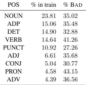
Another interesting finding is that the propor-tion of word to post-edit is the same across the different parts-of-speech (see Table 2).2

Table 1: Number of examples and distribution of labels for the different systems on the training set

System #sent. #words % OK % BAD 1 791 19,456 75.48 24.52 2 621 14,620 59.11 40.89 3 454 11,012 59.76 40.24 4 90 2,296 36.85 63.15 Total 1,956 47,384 64.90 35.10

Table 2: Distribution of labels according to the POS on the training set

POS % in train % BAD NOUN 23.81 35.02

ADP 15.06 35.48 DET 14.90 32.88 VERB 14.64 41.26 PUNCT 10.92 27.26 ADJ 6.61 35.68 CONJ 5.04 30.77 PRON 4.58 43.15 ADV 4.39 36.56

As the classes are unbalanced, prediction per-formance will be evaluated in terms of precision, recall and f1 score computed on the BAD label.

More precisely, if the number of true positive (i.e. 2_{We used FreeLing (http:nlp.lsi.upc.edu/}

freeling/) to predict the POS tags of the translation hypotheses and, for the sake of clarity, mapped the 71 tags used by FreeLing to the 11 universal POS tags of Petrov et al. (2012).

BADword predicted as BAD), false positive (OK word predicted as BAD) and false negative (BAD word predicted as OK) are denoted tp_BAD, fp_BAD and fnBAD, respectively, the quality of a confidence

estimation system is evaluated by the three follow-ing metrics:

pBAD = tpBAD

tp_BAD+fpBAD

(1)

rBAD = _tp tpBAD

BAD+fnBAD (2)

f1 = 2_p·pBAD·rBAD

BAD+rBAD (3)

3 Features

In our experiments, we used 16 features to de-scribe a given target word ti in a translation

hy-pothesist = (tj)m_j=1. To avoid sparsity issues we

decided not to include any lexicalized information such as the word or the previous word identities. As the translation hypotheses were generated by different MT systems, no white-box features (such as word alignment or model scores) are consid-ered. Our features can be organized in two broad categories:

Association Features These features measure the quality of the ‘association’ between the source sentence and a target word: they characterize the probability for a target word to appear in a transla-tion of the source sentence. Two kinds of associa-tion features can be distinguished.

The first one is derived from the lexicalized probabilities p(t|s) that estimate the probability that a source word s is translated by the target wordtj. These probabilities are aggregated using

an arithmetic mean:

p(tj|s) = _n1 n X

i=1

p(tj|si) (4)

wheres = (si)ni=1 is the source sentence (with an

extraNULLtoken). We assume thatp(tj|si) = 0if

the wordstjandsihave never been aligned in the

train set and also consider the geometric mean of the lexicalized probabilities, their maximum value (i.e. maxs∈sp(tj|s)) as well as a binary feature

that fires when the target wordtj is not in the

lex-icalized probabilities table.

pseudo-references to design new MT metrics (Al-brecht and Hwa, 2007; Al(Al-brecht and Hwa, 2008) or for confidence estimation (Soricut and Echi-habi, 2010; Soricut and Narsale, 2012) but, to the best of our knowledge, this is the first time that they are used to predict confidence at the word level.

Pseudo-references are used to define 3 binary features which fire if the target word is in the pseudo-reference, in a2-gram shared between the pseudo-reference and the translation hypothesis or in a common 3-gram, respectively. The lattices representing the search space considered to gen-erate these pseudo-references also allow us to es-timate the posterior probability of a target word that quantifies the probability that it is part of the system output (Gispert et al., 2013). Posteriors ag-gregate two pieces of information for each word in the final hypothesis: first, all the paths in the lat-tice (i.e. the number of translation hypotheses in the search space) where the word appears in are considered; second, the decoder scores of these paths are accumulated in order to derive a confi-dence measure at the word level. In our experi-ments, we considered pseudo-references and lat-tices produced by the n-gram based system de-veloped by our team for last year WMT evalu-ation campaign (Allauzen et al., 2013), that has achieved very good performance.

Fluency Features These features measure the ‘fluency’ of the target sentence and are based on different language models: a ‘traditional’ 4-gram language model estimated on WMT monolingual and bilingual data (the language model used by our system to generate the pseudo-references); a continuous-space 10-gram language model esti-mated with SOUL(Le et al., 2011) (also used by our MT system) and a 4-gram language model based on Part-of-Speech sequences. The latter model was estimated on the Spanish side of the bilingual data provided in the translation shared task in 2013. These data were POS-tagged with FreeLing (Padr´o and Stanilovsky, 2012).

All these language models have been used to de-fine two different features :

• the probability of the word of interestp(tj|h)

where h = tj−1, ..., tj−n+1 is the history

made of then−1previous words or POS

• the ratio between the probability of the sentence and the ‘best’

probabil-ity that can be achieved if the target word is replaced by any other word (i.e. maxv∈Vp(t1, ..., tj−1, v, tj+1, ..., tm) where

the max runs over all the words of the vocabulary).

There is also a feature that describes the back-off behavior of the conventional language model: its value is the size of the largestn-gram of the trans-lation hypothesis that can be estimated by the lan-guage model without relying on back-off probabil-ities.

Finally, there is a feature describing, for each word that appears more than once in the train set, the probability that this word is labeled BAD. This probability is simply estimated by the ratio be-tween the number of times this word is labeled BADand the number of occurrences of this word. It must be noted that most of the features we consider rely on models that are part of a ‘clas-sic’ MT system. However their use for predicting translation quality at the word-level is not straight-forward, as they need to be applied to sentences with a given unknown tokenization. Matching the tokenization used to estimate the model to the one used for collecting the annotations is a tedious and error-prone process and some of the prediction er-rors most probably result from mismatches in tok-enization.

4 Learning Methods 4.1 Classifiers

Predicting whether a word in a translation hypoth-esis should be post-edited or not can naturally be framed as a binary classification task. Based on our experiments in previous campaigns (Singh et al., 2013; Zhuang et al., 2012), we considered ran-dom forest in all our experiments.3

Random forest (Breiman, 2001) is an ensem-ble method that learns many classification trees and predicts an aggregation of their result (for in-stance by majority voting). In contrast with stan-dard decision trees, in which each node is split using the best split among all features, in a ran-dom forest the split is chosen ranran-domly. In spite of this simple and counter-intuitive learning strat-egy, random forests have proven to be very good ‘out-of-the-box’ learners. Random forests have achieved very good performance in many similar 3_{we have used the implementation provided by}

tasks (Chapelle and Chang, 2011), in which only a few dense and continuous features are available, possibly because of their ability to take into ac-count complex interactions between features and to automatically partition the continuous features value into a discrete set of intervals that achieves the best classification performance.

As a baseline, we consider logistic regres-sion (Hastie et al., 2003), a simple linear model where the parameters are estimated by maximiz-ing the likelihood of the trainmaximiz-ing set.

These two classifiers do not produce only a class decision but yield an instance probability that rep-resents the degree to which an instance is a mem-ber of a class. As detailed in the next section, thresholding this probability will allow us to di-rectly optimize the f1 score used to evaluate

pre-diction performance.

4.2 Optimizing the f1 Score

As explained in Section 2, quality prediction will be evaluated in terms of f1 score. The

ing methods we consider can not, as most learn-ing method, directly optimize the f1measure

dur-ing traindur-ing, since this metric does not decompose over the examples. It is however possible to take advantage of the fact that they actually estimate a probability to find the largest f1score on the

train-ing set.

Indeed these probabilities are used with a threshold (usually 0.5) to produce a discrete (bi-nary) decision: if the probability is above the threshold, the classifier produces a positive out-put, and otherwise, a negative one. Each thresh-old value produces a different trade-off between true positives and false positives and consequently between recall and precision: as the the threshold becomes lower and lower, more and more exam-ple are assigned to the positive class and recall in-crease at the expense of precision.

Based on these observations, we propose the following three-step method to optimize the f1

score on the training set:

1. the classifier is first trained using the ‘stan-dard’ learning procedure that optimizes either the 0/1 loss (for random forest) or the likeli-hood (for the logistic regression);

2. all the possible trade-offs between recall and precision are enumerated by varying the threshold; exploiting the monotonicity of

thresholded classifications,4_{this enumeration}

can be efficiently done in O(n·logn) and results in at mostnthreshold values, wheren

is the size of the training set (Fawcett, 2003);

3. all the f1 scores achieved for the different

thresholds found in the previous step are eval-uated; there are strong theoretical guaran-tees that the optimal f1 score that can be

achieved on the training set is one of these values (Boyd and Vandenberghe, 2004).

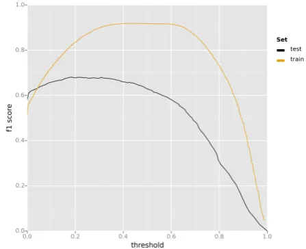
Figure 1 shows how f1score varies with the

deci-sion threshold and allows to assess the difference between the optimal value of the threshold and its default value (0.5).

Figure 1: Evolution of the f1score with respect to

the threshold used to transform probabilities into binary decisions

5 Experiments

The features and learning strategies described in the two previous sections were evaluated on the English to Spanish datasets. As no official devel-opment set was provided by the shared task orga-nizers, we randomly sampled 200 sentences from the training set and use them as a test set through-out the rest of this article. Preliminary experiments show that the choice of this test has a very low im-pact on the classification performance. The dif-ferent hyper-parameters of the training algorithm 4_{Any instance that is classified positive with respect to a}

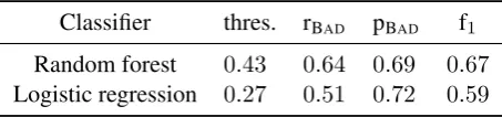
Table 3: Prediction performance for the two learn-ing strategies considered

Classifier thres. rBAD pBAD f1

Random forest 0.43 0.64 0.69 0.67 Logistic regression 0.27 0.51 0.72 0.59

were chosen by maximizing classification perfor-mance (as evaluated by the f1score) estimated on

150 sentences of the training set kept apart as a validation set.

Results for the different learning algorithms considered are presented in Table 3. Random for-est clearly outperforms a simple logistic regres-sion, which shows the importance of using non-linear decision functions, a conclusion at pair with our previous results (Zhuang et al., 2012; Singh et al., 2013).

The overall performance, with a f1 measure of

0.67, is pretty low and in our opinion, not good enough to consider using such a quality estimation system in a computer-assisted post-edition con-text. However, as shown in Table 4, the prediction performance highly depends on the POS category of the words: it is quite good for ‘plain’ words (like verb and nouns) but much worse for other categories.

There are two possible explanations for this observation: predicting the correctness of some morpho-syntaxic categories may be intrinsically harder (e.g. for punctuation the choice of which can be highly controversial) or depend on infor-mation that is not currently available to our sys-tem. In particular, we do not consider any in-formation about the structure of the sentence and about the labels of the context, which may explain why our system does not perform well in predict-ing the labels of determiners and conjunctions. In both cases, this result brings us to moderate our previous conclusions: as a wrong punctuation sign has not the same impact on translation quality as a wrong verb, our system might, regardless of its f1

score, be able to provide useful information about the quality of a translation. This also suggests that we should look for a more ‘task-oriented’ metric.

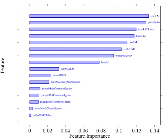
Finally, Figure 2 displays theimportanceof the different features used in our system. Random forests deliver a quantification of the importance of a feature with respect to the predictability of the target variable. This quantification is derived from

Table 4: Prediction performance for each POS tag

System f1

VERB 0.73 PRON 0.72 ADJ 0.70 NOUN 0.69 ADV 0.69 overall 0.67 DET 0.62 ADP 0.61 CONJ 0.57 PUNCT 0.56

the position of a feature in a decision tree: fea-tures used in the top nodes of the trees, which con-tribute to the final prediction decision of a larger fraction of the input samples, play a more impor-tant role than features used near the leaves of the tree. It appears that, as for our previous experi-ments (Wisniewski et al., 2013), the most relevant feature for predicting translation quality is the fea-ture derived from the SOULlanguage model, even if other fluency features seem to also play an im-portant role. Surprisingly enough, features related to the pseudo-reference do not seem to be useful. Further experiments are needed to explain the rea-sons of this observation.

6 Conclusion

In this paper we described the system submitted for Task 2 of WMT’14 Shared Task on Quality Estimation. Our system relies on a binary clas-sifier and consider only a few dense and contin-uous features. While the overall performance is pretty low, a fine-grained analysis of the errors of our system shows that it can predict the quality of plain words pretty accurately which indicates that a more ‘task-oriented’ evaluation may be needed. Acknowledgments

This work was partly supported by ANR project Transread (ANR-12-CORD-0015). Warm thanks to Quoc Khanh Do for his help for training a SOUL model for Spanish.

References

refer-0 0.02 0.04 0.06 0.08 0.1 0.12 0.14 notInIBM1Table

wordNotInSearchSpace pseudoRefCommon3gram pseudoRefCommon1gram pseudoRefCommon2gram

maxMatchingNGramSize geomIBM1

diffMaxLM

bestAl

wordPosterior arithIBM1

posLM tradiLM

maxLMScore priorProba

soulLM

Feature Importance

Feature

Figure 2: Features considered by our system sorted by their relevance for predicting translation errors

ences. InProceedings of the 45th Annual Meeting of the Association of Computational Linguistics, pages 296–303, Prague, Czech Republic, June. ACL.

Joshua Albrecht and Rebecca Hwa. 2008. The role of pseudo references in MT evaluation. In Proceed-ings of the Third Workshop on Statistical Machine Translation, pages 187–190, Columbus, Ohio, June. ACL.

Alexandre Allauzen, Nicolas P´echeux, Quoc Khanh Do, Marco Dinarelli, Thomas Lavergne, Aur´elien Max, Hai-Son Le, and Franc¸ois Yvon. 2013. LIMSI

@ WMT13. In Proceedings of the Eighth Work-shop on Statistical Machine Translation, pages 62– 69, Sofia, Bulgaria, August. ACL.

Stephen Boyd and Lieven Vandenberghe. 2004. Con-vex Optimization. Cambridge University Press, New York, NY, USA.

Leo Breiman. 2001. Random forests. Mach. Learn., 45(1):5–32, October.

Olivier Chapelle and Yi Chang. 2011. Yahoo! learn-ing to rank challenge overview. In Olivier Chapelle, Yi Chang, and Tie-Yan Liu, editors,Yahoo! Learn-ing to Rank Challenge, volume 14 of JMLR Pro-ceedings, pages 1–24. JMLR.org.

Tom Fawcett. 2003. ROC Graphs: Notes and Practical Considerations for Researchers. Technical Report HPL-2003-4, HP Laboratories, Palo Alto.

Adri`a Gispert, Graeme Blackwood, Gonzalo Iglesias, and William Byrne. 2013. N-gram posterior prob-ability confidence measures for statistical machine translation: an empirical study. Machine Transla-tion, 27(2):85–114.

Trevor Hastie, Robert Tibshirani, and Jerome H. Fried-man. 2003. The Elements of Statistical Learning. Springer, July.

Hai-Son Le, Ilya Oparin, Alexandre Allauzen, Jean-Luc Gauvain, and Franc¸ois Yvon. 2011. Structured output layer neural network language model. In Acoustics, Speech and Signal Processing (ICASSP), 2011 IEEE International Conference on, pages 5524–5527. IEEE.

Llu´ıs Padr´o and Evgeny Stanilovsky. 2012. Freeling 3.0: Towards wider multilinguality. InProceedings of the Language Resources and Evaluation Confer-ence (LREC 2012), Istanbul, Turkey, May. ELRA. F. Pedregosa, G. Varoquaux, A. Gramfort, V. Michel,

B. Thirion, O. Grisel, M. Blondel, P. Pretten-hofer, R. Weiss, V. Dubourg, J. Vanderplas, A. Pas-sos, D. Cournapeau, M. Brucher, M. Perrot, and E. Duchesnay. 2011. Scikit-learn: Machine learn-ing in Python. Journal of Machine Learning Re-search, 12:2825–2830.

Slav Petrov, Dipanjan Das, and Ryan McDonald. 2012. A universal part-of-speech tagset. In Proceed-ings of the Eight International Conference on Lan-guage Resources and Evaluation (LREC’12), Istan-bul, Turkey, may. European Language Resources Association (ELRA).

via ranking. In Proceedings of the 48th Annual Meeting of the Association for Computational Lin-guistics, pages 612–621, Uppsala, Sweden, July. ACL.

Radu Soricut and Sushant Narsale. 2012. Combining quality prediction and system selection for improved automatic translation output. InProceedings of the Seventh Workshop on Statistical Machine Transla-tion, pages 163–170, Montr´eal, Canada, June. ACL. Guillaume Wisniewski, Anil Kumar Singh, and Franc¸ois Yvon. 2013. Quality estimation for ma-chine translation: Some lessons learned. Machine Translation, 27(3).