Extrinsic Evaluation of Dialog State Tracking and Predictive Metrics
for Dialog Policy Optimization
Sungjin Lee
Language Technologies Institute,
Carnegie Mellon University,
Pittsburgh, Pennsylvania, USA
[email protected]
Abstract
During the recent Dialog State Tracking Challenge (DSTC), a fundamental question was raised: “Would better performance in
dialog state tracking translate to better performance of the optimized policy by reinforcement learning?” Also, during the challenge system evaluation, another non-trivial question arose: “Which evaluation
metric and schedule would best predict improvement in overall dialog performance?”
This paper aims to answer these questions by applying an off-policy reinforcement learning method to the output of each challenge system. The results give a positive answer to the first question. Thus the effort to separately improve the performance of dialog state tracking as carried out in the DSTC may be justified. The answer to the second question also draws several insightful conclusions on the characteristics of different evaluation metrics and schedules.
1
Introduction
Statistical approaches to spoken dialog management have proven very effective in gracefully dealing with noisy input due to
Automatic Speech Recognition (ASR) and
Spoken Language Understanding (SLU) error (Lee, 2013; Williams et al., 2013). Most recent advances in statistical dialog modeling have been based on the Partially Observable Markov Decision Processes (POMDP) framework which provides a principled way for sequential action planning under uncertainty (Young et al., 2013). In this approach, the task of dialog management is generally decomposed into two subtasks, i.e., dialog state tracking and dialog policy learning. The aim of dialog state tracking is to accurately
estimate the true dialog state from noisy observations by incorporating patterns between turns and external knowledge as a dialog unfolds (Fig. 1). The dialog policy learning process then strives to select an optimal system action given the estimated dialog state.
Many dialog state tracking algorithms have been developed. Few studies, however, have reported the strengths and weaknesses of each method. Thus the Dialog State Tracking Challenge (DSTC) was organized to advance state-of-the-art technologies for dialog state tracking by allowing for reliable comparisons between different approaches using the same datasets (Williams et al., 2013). Thanks to the DSTC, we now have a better understanding of effective models, features and training methods we can use to create a dialog state tracker that is not only of superior performance but also very robust to realistic mismatches between development and deployment environments (Lee and Eskenazi, 2013).
Despite the fruitful results, it was largely limited to intrinsic evaluation, thus leaving an important question unanswered: “Would the improved performance in dialog state tracking carry over to dialog policy optimization?”
Furthermore, there was no consensus on what and when to measure, resulting in a large set of metrics being evaluated with three different schedules. With this variety of metrics, it is not clear what the evaluation result means. Thus it is important to answer the question: “Which metric best serves as a predictor to the improvement in dialog policy optimization” since this is the ultimate goal, in terms of end-to-end dialog performance. The aim of this paper is to answer these two questions via corpus-based experiments. Similar to the rationale behind the DSTC, the corpus-based design allows us to
compare different trackers on the same data. We applied a sample efficient off-policy reinforcement learning (RL) method to the outputs of each tracker so that we may examine the relationship between the performance of dialog state tracking and that of the optimized policy as well as which metric shows the highest correlation with the performance of the optimized policy.
This paper is structured as follows. Section 2 briefly describes the DSTC and the metrics adopted in the challenge. Section 3 elaborates on the extrinsic evaluation method based on off-policy RL. Section 4 presents the extrinsic evaluation results and discusses its implication on metrics for dialog state tracking evaluation. Finally, Section 5 concludes with a brief summary and suggestions for future research.
2
DSTC Task and Evaluation Metrics
This section briefly describes the task for the DSTC and evaluation metrics. For more details, please refer to the DSTC manual1.
1
http://research.microsoft.com/apps/pubs/?id=169024
2.1 Task Description
DSTC data is taken from several different spoken dialog systems which all provided bus schedule information for Pittsburgh, Pennsylvania, USA (Raux et al., 2005) as part of the Spoken Dialog Challenge (Black et al., 2011). There are 9 slots which are evaluated: route,
from.desc, from.neighborhood, from.monument,
to.desc, to.neighborhood, to.monument, date, and
time. Since both marginal and joint representations of dialog states are important for deciding dialog actions, the challenge takes both into consideration. Each joint representation is an assignment of values to all slots. Thus there are 9 marginal outputs and 1 joint output in total, which are all evaluated separately.
[image:2.595.73.514.84.292.2]scores is restricted to sum to 1.0. Thus 1.0 – total score is defined as the score of a special value
None that indicates the user’s goal has not yet appeared on any SLU output.
2.2 Evaluation Metrics
To evaluate tracker output, the correctness of each hypothesis is labeled at each turn. Then hypothesis scores and labels over the entire dialogs are collected to compute 11 metrics:
Accuracy measures the ratio of states under evaluation where the top hypothesis is correct.
ROC.V1 computes the following quantity:
( ) ( )
where is the total number of top hypotheses over the entire data and ( )
denotes the number of correctly accepted top hypotheses with the threshold being set to . Similarly FA denotes false-accepts and FR false-rejects. From these quantities, several metrics are derived. ROC.V1.EER computes FA.V1(s) where FA.V1(s) = FR.V1(s). The metrics ROC.V1.CA05,
ROC.V1.CA10, and ROC.V1.CA20
compute CA.V1(s) when FA.V1(s) = 0.05, 0.10, and 0.20 respectively. These metrics measure the quality of score via plotting accuracy with respect to false-accepts so that they may reflect not only accuracy but also discrimination.
ROC.V2 computes the conventional ROC quantity:
( ) ( ) ( )
ROC.V2.CA05, ROC.V2.CA10, and
ROC.V2.CA20 do the same as the V1 versions. These metrics measure the discrimination of the score for the top hypothesis independently of accuracy.
Note that Accuracy and ROC curves do not take into consideration non-top hypotheses while the following measures do.
L2 calculates the Euclidean distance between the vector consisting of the scores of all hypotheses and a zero vector with 1 in
the position of the correct one. This measures the quality of tracker’s output score as probability.
AvgP indicates the averaged score of the correct hypothesis. Note that this measures the quality of the score of the correct hypothesis, ignoring the scores assigned to incorrect hypotheses.
MRR denotes the mean reciprocal rank of the correct hypothesis. This measures the quality of rank instead of score.
As far as evaluation schedule is concerned, there are three schedules for determining which turns to include in each evaluation.
Schedule 1: Include all turns. This schedule allows us to account for changes in concepts that are not in focus. But this makes across-concept comparison invalid since different concepts appear at different times in a dialog. Schedule 2: Include a turn for a given
concept only if that concept either appears on the SLU N-Best list in that turn, or if the system’s action references that concept in that turn. Unlike schedule 1, this schedule makes comparisons across concepts valid but cannot account for changes in concepts which are not in focus.
Schedule 3: Include only the turn before the system starts over from the beginning, and the last turn of the dialog. This schedule does not consider what happens during a dialog.
3
Extrinsic Evaluation Using Off-Policy
Reinforcement Learning
In this section, we present a corpus-based method for extrinsic evaluation of dialog state tracking. Thanks to the corpus-based design where outputs of various trackers with different characteristics are involved, it is possible to examine how the differences between trackers affect the performance of learned policies. The performance of a learned policy is measured by the expected return at the initial state of a dialog which is one of the common performance measures for episodic tasks.
3.1 Off-Policy RL on Fixed Data
system’s behavior is called Behavior policy. As far as a specific algorithm is concerned, we have adopted Least-Squares Temporal Difference
(LSTD) (Bradtke and Barto, 1996) for policy evaluation and Least-Squares Policy Iteration
(LSPI) (Lagoudakis and Parr, 2003) for policy learning. LSTD and LSPI have been well known to be sample efficient, thus easily lending themselves to the application of RL to fixed data (Pietquin et al., 2011). LSPI is an instance of
Approximate Policy Iteration where an approximated action-state value function (a.k.a Q function) is established for a current policy and an improved policy is formed by taking greedy actions with respect to the estimated Q function. The process of policy evaluation and improvement iterates until convergence. For value function approximation, in this work, we adopted the following linear approximation architecture:
̂ ( ) ( )
where is the set of parameters, ( ) an activation vector of basis functions, a state and an action. Given a policy and a set of state transitions ( ) , where is the
reward that the system would get from the environment by executing action at state , the approximated state-action value function ̂
is estimated by LSTD. The most important part of LSTD lies in the computation of the gradient of temporal difference:
( ) ( ( ))
In LSPI, ( ) takes the form of greedy policy:
( ) ̂ ( )
It is however critical to take into consideration the inherent problem of insufficient exploration in fixed data to avoid overfitting (Henderson et al., 2008). Thus we confined the set of available actions at a given state to the ones that have an occurrence probability greater than some threshold :
( )
( | ) ̂
( )
The conditional probability ( | ) can be easily estimated by any conventional
classification methods which provide posterior probability. In this study, we set to 0.1.
3.2 State Representation and Basis Function
In order to make the process of policy optimization tractable, the belief state is normally mapped to an abstract space by only taking crucial information for dialog action selection, e.g., the beliefs of the top and second hypotheses for a concept. Similarly, the action space is also mapped into a smaller space by only taking the predicate of an action. In this work, the simplified state includes the following elements:
The scores of the top hypothesis for each concept with None excluded
The scores of the second hypothesis for each concept with None excluded
The scores assigned to None for each concept
Binary indicators for a concept if there are hypotheses except None
The values of the top hypothesis for each concept
A binary indicator if the user affirms when the system asks a yes-no question for next bus
It has been shown that the rapid learning speed of recent approaches is partly attributed to the use of kernels as basis functions (Gasic et al., 2010; Lee and Eskenazi, 2012; Pietquin et al., 2011). Thus to make the best of the limited amount of data, we adopted a kernelized approach. Similar to previous studies, we used a product of kernel functions:
( ) ( ) ∏ ( )
where ( ) is responsible for a vector of continuous elements of a state and ( ) for each discrete element. For the continuous elements, we adopted Gaussian kernels:
( ) ( ‖ ‖
)
respectively. For a discrete element, we adopted delta kernel:
( ) ( )
where ( ) returns one if , zero otherwise and represents an element of a state. As the number of data points increases, kernelized approaches commonly encounter severe computational problems. To address this issue, it is necessary to limit the active kernel functions being used for value function approximation. This sparsification process has to find out the sufficient number of kernels which keeps a good balance between computational tractability and approximation quality. We adopted a simple sparsification method which was commonly used in previous studies (Engel et al., 2004). The key intuition behind of the sparsification method is that there is a mapping
( ) to a Hilbert space in which the kernel function ( ) is represented as the inner product of ( ) and ( ) by the Mercer’s theorem. Thus the kernel-based representation of Q function can be restated as a plain linear equation in the Hilbert space:
̂ ( ) ∑ ( ) 〈 ( ) ∑ ( )〉
where denotes the pair of state and action. The term ∑ ( ) plays the role of the weight vector in the Hilbert space. Since this term takes the form of linear combination, we can safely remove any linearly dependent ( ) without changing the weighted sum by tuning . It is known that the linear dependence of ( ) from the rest can be tested based on kernel functions as follows:
( ) ( ) (1)
where ( ) ( )
and is a sparsification threshold. When equation 1 is satisfied, can be safely removed from the set of basis functions. Thus the sparsity can be controlled by changing . It can be shown that equation 1 is minimized when
( ), where is the Gram matrix
excluding . In the experiments, was set to 3.
3.3 Reward Function
The reward function is defined following a common approach to form-filling, task-oriented systems:
Every correct concept filled is rewarded 100 Every incorrect concept filled is assigned
-200
Every empty concept is assigned -300 if the system terminated the session, -50 otherwise. At every turn, -20 is assigned
The reward structure is carefully designed such that the RL algorithm cannot find a way to maximize the expected return without achieving the user goal.
4
Experimental Setup
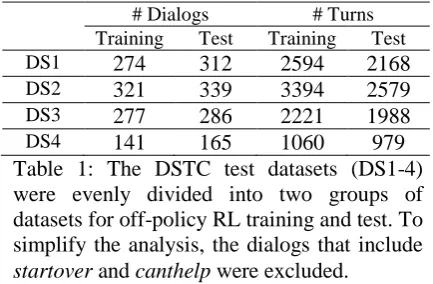
In order to see the relationship between the performance of dialog state tracking and that of the optimized policy, we applied the off-policy RL method presented in Section 3 to the outputs of each tracker for all four DSTC test datasets2. The summary statistics of the datasets are presented in Table 1. In addition, to quantify the impact of dialog state tracking on an end-to-end dialog, the performance of policies optimized by RL was compared with Behavior policies and another set of learned policies using supervised learning (SL). Note that Behavior policies were developed by experts in spoken dialog research. The use of a learned policy using supervised
2 We took the entry from each team that achieved the
highest ranks of that team in the largest number of evaluation metrics: entry2 for team3 and team6, entry3 for team8, entry4 for team9, and entry1 for the rest of the teams. We were not, however, able to process the tracker output of team2 due to its large size. This does not negatively impact the general results of this paper.
# Dialogs # Turns
Training Test Training Test
DS1 274 312 2594 2168
DS2 321 339 3394 2579
DS3 277 286 2221 1988
DS4 141 165 1060 979
Table 1: The DSTC test datasets (DS1-4) were evenly divided into two groups of datasets for off-policy RL training and test. To simplify the analysis, the dialogs that include
[image:5.595.305.522.74.216.2]learning (Hurtado et al., 2005) is also one of the common methods of spoken dialog system development. We exploited the SVM method with the same kernel functions as defined in Section 3.2 except that the action element is not included. The posterior probability of the SVM model was also used for handling the insufficient exploration problem (in Section 3.1).
5
Results and Discussion
The comparative results between RL, SL and Behavior policies are plotted in Fig. 2. Despite the relatively superior performance of SL policies over Behavior policies, the performance improvement is neither large nor constant. This confirms that Behavior policies are very strong baselines which were designed by expert researchers. RL policies, however, consistently outperformed Behavior as well as SL policies, with a large performance gap. This result indicates that the policies learned by the proposed off-policy RL method are a lot closer to optimal ones than the hand-crafted policies created by human experts. Given that many state features are derived from the belief state, the large improvement in performance implies that the estimated belief state is indeed a good summary representation of a state, maintaining the Markov property between states. The Markov
property is a crucial property for RL methods to approach to the optimal policy. On the other hand, most of the dialog state trackers surpassed the baseline tracker (team0) in the performance
of RL policies. This result assures that the better the performance in dialog state tracking, the better a policy we can learn in the policy optimization stage. Given these two results, we can strongly assert that dialog state tracking plays a key role in enhancing end-to-end dialog performance.
Another interesting result worth noticing is that the performance of RL policies does not exactly align with the accuracy measured at the end of a dialog (Schedule 3) which would have been the best metric if the task were a one-time classification (Fig. 2). This misalignment therefore supports the speculation that accuracy-schedule3 might not be the most appropriate metric for predicting the effect of dialog state tracking on end-to-end dialog performance. In order to better understand What To Measure and
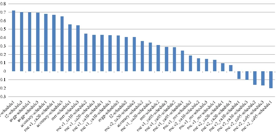
When To Measure to predict end-to-end dialog performance, a correlation analysis was carried out between the performance of RL policies and that of the dialog state tracking measured by different metrics and schedules. The correlations are listed in descending order in Fig. 3. This result reveals several interesting insights for different metrics.
[image:6.595.145.454.75.290.2]terminates the session, to refine its belief state when there is no dominant hypothesis. Thus accurate estimation of the beliefs of all observed hypotheses is essential. This is why the evaluation of only the top hypothesis does not provide sufficient information.
Second, schedule1 and schedule3 showed a stronger correlation than schedule2. In fact schedule2 was more preferred in previous studies since it allows for a valid comparison of different concepts (Williams, 2013; Williams et al., 2013). This result can be explained by the fact that the best system action is selected by considering all of the concepts together. For example, when the system moves the conversation focus from one concept to another, the beliefs of the concepts that are not in focus are as important as the concept in focus. Thus evaluating all concepts at the same time is more suitable for predicting the performance of a sequential decision-making task involving multiple concepts in its state.
Finally, metrics for evaluating discrimination quality (measured by ROC.V2) have little correlation with end-to-end dialog performance. In order to understand this relatively unexpected result, we need to give deep thought to how the scores of a hypothesis are distributed during the session. For example, the score of a true hypothesis usually starts from a small value due to the uncertainty of ASR output and gets bigger every time positive evidence is observed. The score of a false hypothesis usually stays small or medium. This leads to a situation where both true
and false hypotheses are pretty much mixed in the zone of small and medium scores without significant discrimination. It is, however, very important for a metric to reveal a difference between true and false hypotheses before their scores fully arrive at sufficient certainty since most additional turns are planned for hypotheses with a small or medium score. Thus general metrics evaluating discrimination alone are hardly appropriate for a tracking problem where the score develops gradually. Furthermore, the choice of threshold (i.e. FA = 0.05, 0.10, 0.20) was made to consider relatively unimportant regions where the true hypothesis is likely to have a higher score, meaning that no further turns need to be planned.
6
Conclusion
In this paper, we have presented a corpus-based study that attempts to answer two fundamental questions which, so far, have not been rigorously addressed: “Would better performance in dialog state tracking translate to better performance of the optimized policy by RL?” and “Which evaluation metric and
[image:7.595.76.523.77.291.2]with the performance of optimized policies were computed. The results revealed several insightful conclusions: 1) Metrics measuring score quality are more suitable for predicting the performance of an optimized policy. 2) Evaluation of all concepts at the same time is more appropriate for predicting the performance of a sequential decision making task involving multiple concepts in its state. 3) Metrics evaluating only discrimination (e.g., ROC.V2) are inappropriate for a tracking problem where the score gradually develops. Interesting extensions of this work include finding a composite measure of conventional metrics to obtain a better predictor. A data-driven composition may tell us the relative empirical importance of each metric. In spite of several factors which generalize our conclusions such as handling insufficient exploration, the use of separate test sets and various mismatches between test sets, it is still desirable to run different policies for live tests in the future. Also, since the use of an approximate policy evaluation method (e.g. LSTD) can introduce systemic errors, more deliberate experimental setups will be designed for a future study: 1) the application of different RL algorithms for training and test datasets 2) further experiments on different datasets, e.g., the datasets for DSTC2 (Henderson et al., 2014). Although the state representation adopted in this work is quite common for most systems that use a POMDP model, different state representations could possibly reveal new insights.
References
A. Black et al., 2011. Spoken dialog challenge 2010: Comparison of live and control test results. In Proceedings of SIGDIAL.
S. Bradtke and A. Barto, 1996. Linear Least-Squares algorithms for temporal difference learning. Machine Learning, 22, 1-3, 33-57.
Y. Engel, S. Mannor and R. Meir, 2004. The Kernel Recursive Least Squares Algorithm. IEEE Transactions on Signal Processing, 52:2275-2285.
M. Gasic and S. Young, 2011. Effective handling of dialogue state in the hidden information state POMDP-based dialogue manager. ACM Transactions on Speech and Language Processing, 7(3).
M. Gasic, F. Jurcicek, S. Keizer, F. Mairesse, B. Thomson, K. Yu and S. Young, 2010. Gaussian Processes for Fast Policy Optimisation of
POMDP-based Dialogue Managers, In Proceedings of SIGDIAL, 2010.
J. Henderson, O. Lemon and K. Georgila, 2008. Hybrid reinforcement/supervised learning of dialogue policies from fixed data sets. Computational Linguistics, 34(4):487-511.
M. Henderson, B. Thomson and J. Williams, 2014. The Second Dialog State Tracking Challenge. In Proceedings of SIGDIAL, 2014.
L. Hurtado, D. Grial, E. Sanchis and E. Segarra, 2005. A Stochastic Approach to Dialog Management. In Proceedings of ASRU, 2005.
M. Lagoudakis and R. Parr, 2003. Least-squares policy iteration. Journal of Machine Learning Research 4, 1107-1149.
S. Lee, 2013. Structured Discriminative Model For Dialog State Tracking. In Proceedings of SIGDIAL, 2013.
S. Lee and M. Eskenazi, 2012. Incremental Sparse Bayesian Method for Online Dialog Strategy Learning. IEEE Journal of Selected Topics in Signal Processing, 6(8).
S. Lee and M. Eskenazi, 2013. Recipe For Building Robust Spoken Dialog State Trackers: Dialog State Tracking Challenge System Description. In Proceedings of SIGDIAL, 2013.
O. Pietquin, M. Geist, S. Chandramohan and H. Frezza-buet, 2011. Sample Efficient Batch Reinforcement Learning for Dialogue Management Optimization. ACM Transactions on Speech and Language Processing, 7(3).
O. Pietquin, M. Geist, and S. Chandramohan, 2011. Sample Efficient On-Line Learning of Optimal Dialogue Policies with Kalman Temporal Differences. In Proceedings of IJCAI, 2011.
A. Raux, B. Langner, D. Bohus, A. W Black, and M. Eskenazi, 2005. Let’s Go Public! Taking a Spoken Dialog System to the Real World. In Proceedings of Interspeech.
J. Williams, 2013. Multi-domain learning and generalization in dialog state tracking. In Proceedings of SIGDIAL, 2013.
J. Williams, A. Raux, D. Ramachandran and A. Black, 2013. The Dialog State Tracking Challenge. In Proceedings of SIGDIAL, 2013.