Munich Personal RePEc Archive
The environmental Kuznets curve in a
public spending model of economic
growth
Diallo, Ibrahima Amadou
Centre d’Etudes et de Recherches sur le Développement
International, CERDI
9 June 2014
Online at
https://mpra.ub.uni-muenchen.de/56528/
The Environmental Kuznets Curve in a Public
Spending Model of Economic Growth
Ibrahima Amadou Diallo
∗June 9, 2014
Abstract
This paper theoretically analyzes the dynamics of economic growth and the environmental
Kuznets curve. This curve states an inverse U-relationship between pollution and income. The
presented model specifically shows how a dynamic environmental Kuznets curve can emerge
by introducing pollution and abatement technology in a public spending model of endogenous
economic growth. We also derive the turning point in function of the parameters of the model.
The numerical section demonstrates that when taxes are below some threshold, the turning point
decreases with taxes but it increases when taxes are above the threshold point given some
ex-planations about an N-shaped Kuznets curve. Additionally, the simulations demonstrate that
taxes reduce the level of pollution by pulling down the environmental Kuznets curve. Lastly the
numerical exercises highlight that the pollution level of the social planner problem is less than
that of the representative agent.
Keywords:Abatement; Dynamic Optimization; Endogenous Growth Theory; Environmental Kuznets Curve;
Nu-merical Simulations; Pollution; Public Spending; Taxes; Turning Point
JEL Classification:C61, C63, H23, H41, H54, H61, O41, O44
∗Clermont University, University of Auvergne, Centre d’ ´Etudes et de Recherches sur le D´eveloppement
International, CERDI-CNRS, 65 bd Franc¸ois Mitterrand, 63000 Clermont-Ferrand, France. Author’s contact:
1
Introduction
In the last three decades, the issues of environmental degradation have increasingly attracted the attention of scientists, the media, politicians and citizens worldwide. The main reasons for this consideration are global warming, environmental pollution, global climate change. . . This is why in recent years the question of sustainable development has gained an increasing popularity among people with various backgrounds. Sustainable development can be defined as a mean of achieving both economic development and the viability of the environment. Economists also have been participating in this debate on sustainable development. Since the early 1990s the environmental Kuznets curve (henceforth EKC) plays a central role in the studies of economists about the environment. The EKC states an inverse U-link between pollution (environmental degradation) and GDP per capita. The intuition behind the EKC is that in the early stages of development, when income per capita is not very high and is below some threshold (turning point), there is little concern for the environment and pollution increases with income. But when the income augments sufficiently and is above the turning point, worries for the
environment rise and environmental degradation starts to decrease when GDP per capita expands. It was Panayotou (1993) who first invented the name“Environmental Kuznets Curve”. The term“Kuznets Curve”itself dates back to Kuznets (1955) who observed that there exist a reverse U-shape connection between income inequality and GDP per capita. Grossman (1995) identifies three different ways in which economic growth acts on
en-vironmental quality: the scale effect, the composition effect and the technique effect. The
scale effect is caused by the fact that as the economy develops; its scale becomes large and
leads to environmental degradation. This happens because large output implies the use of more inputs and natural resources in the production process. The huge output causes more pollution as a consequence of the economic activity and leads to environmental degradation in the end. The composition effect states that GDP growth can have a
posi-tive effect on environmental quality. Panayotou (1993) underlines that pollution starts to
augment as the structure of the economy shifts from agricultural to industrial production but decreases when this structure changes from energy intensive industries to services and to technology-demanding industries. The technique effect postulates that growing
which normally leads to the replacement of obsolete and dirty technologies with cleaner ones which in turn contributes to the amelioration of the environment. Consequently, the inverted U-relationship of the EKC might be the result of these three effects combined
together. In the early stages of economic development, the scale effect tends to dominate
and we witness an environmental degradation in the economy. But at later phases of growth, the composition and the technique effects will eventually prevail and we observe
a reduction of the pollution level in the country.
The EKC started as an empirical research phenomenon at the beginning of the 1990s. Most of the pioneering studies find out the existence of an inverse U-link between various environmental degradation indicators (SO2,CO2,NOx,. . . ) and income per capita. The
first study on the EKC was that of Grossman and Krueger (1991) while examining the environmental consequences of the North American free trade agreement. Using a sample of study of 42 countries, they discovered that smoke and SO2 augment with
GDP per capita at low levels of income but they diminish with economic growth at higher levels of wealth. Employing panel data techniques on a representative sample of countries, Grossman and Krueger (1995) find an EKC for fecal pollution of waterway beds, the state of the oxygen regulation in river beds, pollution of watercourse beds by heavy metals and urban air contamination with turning points occurring before the countries of the sample reach 8000 American dollars. Shafik and Bandyopadhyay (1992) discover that there exist a Kuznets curve for the deforestation, the SO2, and carbon emissions
with turning point around 2000, 3000 and 4000 constant 1985 US dollars respectively. Selden and Song (1994) using the same data sources as Grossman and Krueger (1993) and Grossman and Krueger (1995) show the presence of an EKC with high turning points1 for two environmental degradation indicators (SO2 and suspended particulate
matter). Hill and Magnani (2002) using cross-section data show that there exist an EKC with high turning points forCO2 for each of the following years: 1970, 1980 and 1990.
Berrens, Bohara, Gawande and Wang (1997) find a reverse U-curve for municipal waste for the USA with a threshold near 20000 dollars by employing a flexible generalized gamma function as a replacement of the common polynomial specification. Despite the overwhelming presence of empirical studies on the existence of the EKC, there are
some researchers that have found the opposite results. For instance, Halkos and Tsionas (2001), using regime switching models on a cross-section of developing and developed countries, discover an increasing relationship between two pollution indicators (CO2and
deforestation), and income. Roca and Alc´antara (2001) examine the EKC for Spain from 1972 to 1997. They also find no evidence of an inverse U-connection forCO2.
The EKC has also been studied theoretically. John and Pecchenino (1994) use a general equilibrium overlapping generations model to analyze the pollution-income relationship. In their model each agent lives two periods. The model shows that at early stages of development, the economy has little capital and agents at initial generations spend no money on the environment. As a consequence the environment deteriorates. After some point in time, capital stock starts to gather and income turns out to be higher. This makes that agents at later generations start to take care of the environment. This situation thus generates an inverted U-shape curve between environmental degradation and revenue. Selden and Song (1995) illustrate that an EKC for pollution can emerge in a neoclassical growth model. The model demonstrates that when pollution is not very high, the agents pay no money to preserve the environment and toxic wastes increase. But when environmental degradation attains a certain threshold, the agents reconsider their policy and devote more resources to protect the environment and pollution decreases. Stokey (1998) utilizes economic growth models in which production depends on pollution and usual inputs. The dirtiest technology is used if production is below the turning point and pollution augments with wealth. Above the turning point cleaner techniques are employed and pollution diminishes if the elasticity of the marginal utility of consumption goods is greater than one. Andreoni and Levinson (2001) studies a static utility function only model in which happiness depends positively with consumption and negatively with pollution. They find that if abatement satisfies the increasing returns to scales property, an EKC emerges without considering production functions. In their model the EKC is the result of two combined processes. When revenue is small, consumption is also small and the impact of abatement effort has a minor effect on environment giving
because consumption is large. Also the effect of abatement on happiness is huge given
the increasing returns nature of abatement. Consequently, the agent spends more money on abatement and environmental degradation decreases. Dinda (2005) also proposes a model that explains the emergence of the EKC according, approximately, to the previous explanations. Egli and Steger (2007) prolong the model of Andreoni and Levinson (2001) in the context of a dynamic AK economic growth model. Their model shows that an EKC arises in a dynamic situation when the abatement technology obeys the increasing returns to scales property. Furthermore, they analyze the determinants of the turning point and the time to attain this point. Their model also gives a possible description for the appearance of an N-shaped pollution-income curve. Brock and Taylor (2004) analyze an augmented Solow model2in which production is distributed between abatement and consumption. In their numerical simulations they illustrate that, in the optimal path, the ratio of environmental degradation to GDP per capita initially augments and then diminishes. Using the real options approach, Kijima, Nishide and Ohyama (2011) show how aΛshape and an N-shaped Kuznets curve can emerge in a unified structure.
Similar to the works in the previous paragraph, this paper theoretically studies how the EKC forms. It is an extension of Andreoni and Levinson (2001) model in a dynamic endogenous growth setting. But unlike Egli and Steger (2007) who examine theAKcase, we in this paper analyze the EKC in a public spending model of endogenous economic growth`a laBarro (1990). The model studied here can thus be considered as an extension to both the Andreoni and Levinson (2001) and Barro (1990) models. Consequently, the main contribution of the paper is to have shown how a dynamic environmental Kuznets curve can emerge by introducing pollution and abatement technology in a public spending model of endogenous economic growth. The results show that, under the increasing returns to scales property of abatement, an EKC appears in our dynamic endogenous growth model. We also derive the turning point in function of the parameters of the model. The numerical section demonstrates that this turning point decreases when taxes increase and are below some threshold. Above this threshold the turning point starts to augment given some explanations for the possible existence of an N-shaped Kuznets curve. Moreover, the simulations reveal that taxes reduce the level of pollution by pulling
down the EKC. Finally the numerical exercises illustrate that the pollution level of the social planner problem is less than that of the representative agent.
2
Theoretical Framework
In this section, we present the theoretical model and show how all important equations are obtained.
2.1
Setting the Model
As stated in the introduction, our model is an extension of both Andreoni and Levinson (2001), and Barro (1990) models. The model presumes identical individuals meaning that they have similar preference parameters. Therefore we can employ the representative-agent hypothesis within which the analysis is done from the decisions of one representative-agent. The individual selects consumptionC(t) and abatementE(t) paths that maximizes the present value of his lifetime utility function3subject to some constraints and the initial value of capital.
Max{C(t),E(t)}U(0)=
Z ∞
0
e−ρtln (C(t)−zP(t))dt (1) Subject to:
P(t)=C(t)−C(t)ηE(t)θGC(t)φ (2)
GI(t)+GC(t)+TF(t)=TR(t) (3)
TR(t)=τY(t) (4)
Y(t)=AK(t)1−αGI(t)α (5)
Y(t)−τY(t)+TF(t)=C(t)+IV(t)+E(t) (6)
d
dtK(t)=IV(t)−δK(t) (7)
GC(t)=ψGI(t) (8)
TF(t)=υTR(t) (9)
And
K(0) is given
In equation (1), C(t) is consumption, E(t) is abatement, ρ represents the subjective rate of time preference. It is assumed thatρis positive. P(t) is pollution andz >0 de-notes a weight associated to environmental degradation in the utility function. P(t) >0 since pollution is a flow, we cannot have negative pollution and we are interested only in interior solutions. The instantaneous utility functionu(C(t),P(t)) = ln (C(t)−zP(t))
is logarithmic. This functional form allows us to find closed form solutions for the dynamic variables and the EKC. This functional specification is a nonlinear version of Andreoni and Levinson (2001) utility function. It has also been considered by Egli and Steger (2007). We have C(t) > zP(t). Furthermore we need the following condi-tions for the felicity function: ∂C∂(t)u(C(t),P(t)) =(C(t)−zP(t))−1 >0; ∂2
∂C(t)2u(C(t),P(t)) =
−(C(t)−zP(t))−2 <0; ∂P∂(t)u(C(t),P(t)) =− z
C(t)−zP(t) <0;
∂2
∂P(t)2u(C(t),P(t)) =−
z2
(C(t)−zP(t))2 <
0; ∂C(t∂)2∂P(t)u(C(t),P(t)) = z
(C(t)−zP(t))2 > 0. The first two equalities show that
instanta-neous utility increases with consumption and marginal utility is decreasing in regard to consumption. The following two conditions demonstrate that the felicity function diminishes with pollution and the marginal utility of pollution is declining as well. The last expression illustrates that pollution augment with the marginal utility of consump-tion. In the equations, we ensure that υ, ψ, η, θ, φ, α, τ andδ ∈ (0,1). Equality (2) says that pollution,P(t), augments with consumption but diminishes with consumption, abatement and government consumption,GC(t). It is an improved version of Andreoni and Levinson (2001) environmental degradation equation. We add to their framework, the fact that government consumption acts on pollution. Throughout the paper we as-sume thatη+θ+φ > 1. This assumption allows us get an EKC and is the increasing
non-excludable public good. This specification has similarly been investigated by Barro (1990). In equality (6) the left hand side is the total resources of the household and the right hand side his total expenditures. The household resources come from disposable income,Y(t)−τY(t), and transfers received,TF(t). The family then uses his wealth to buy consumption,C(t), invest inIV(t) and spend on pollution abatement,E(t). Equation (7) denotes the law of motion of physical capital stock. It states that capital accumulation,
d
dtK(t), comes from investment,IV(t), from which we deduct depreciated capital,δK(t).
In the next two equalities ( (8) and (9)) government consumption,GC(t) and transfers,
TF(t), are constant fractions of government investment,GI(t), and total revenue,TR(t), respectively. The last expression tells us that initial capital stock,K(0), is given. Labor supply is inelastic and constant. We assumeL(t)=1, thus all variables are expressed in
per capita term. We also neglect wages coming from labor.
2.2
Formation of the Resource Constraint
In this subsection, we will show how the resource constraint is obtained. Substitute transfers and total revenue from equations (9) and (4) respectively in equality (6). Collect terms and get:
(υ τ−τ+1)Y(t)=C(t)+IV(t)+E(t) (10)
Replacing output by its value and pulling out investment we have:
IV(t)=(υ τ−τ+1)AK(t)1−αGI(t)α−C(t)−E(t) (11)
Substitute this last expression in (7) and obtain the final law of motion of capital stock:
d
dtK(t)=(υ τ−τ+1)AK(t)
1−αGI(t)α−C(t)−E(t)−δK(t) (12)
2.3
Economic Equilibrium
u(C(t),P(t))=ln (C(t)−zP(t)) (13)
If we substitute pollution by its value from (2) into (13) and setz =1, we find after
some algebra:
u(·)=lnC(t)ηE(t)θψφGI(t)φ (14)
This equality reveals that instantaneous utility increases with consumption, abate-ment and productive governabate-ment spending. Given this result, the present value Hamil-tonian,H(·), of the representative agent is:
(15)
H(·)=e−ρtlnC(t)ηE(t)θψφGI(t)φ
+µ(t)(υ τ−τ+1)AK(t)1−αGI(t)α−C(t)−E(t)−δK(t)
The variableµ(t) is the costate variable. The first order conditions for this problem are:
The derivative of the Hamiltonian with respect to consumption.
e−ρtη
C(t) −µ(t)=0 (16) The derivative of the Hamiltonian with respect to abatement.
e−ρtθ
E(t) −µ(t)=0 (17) We take the derivative of the Hamiltonian with regard to the state variable, set it equal to the negative of the derivative of the costate variable relative to time and rearrange the equation to get.
d
dtµ(t)=−µ(t)
(υ τ−τ+1) (1−α)AK(t)−αGI(t)α−δ (18)
Combining equations (16) and (17), and simplifying we have:
C(t)
E(t) =
η
We can isolateµ(t) from equality (16), take the natural logarithm of both sides, derive the resulting expression with respect to time and get:
d dtµ(t)
µ(t) =−ρ−
d dtC(t)
C(t) (20)
If we join equations (18)and (20), and continue with some more algebra, we find:
d dtC(t)
C(t) =(υ τ−τ+1) (1−α)AK(t)
−αGI(t)α−δ−ρ (21)
Substituting government consumption, transfers and total revenue from equations (8), (9) and (4) respectively in equally (3) and reorganizing, we have:
1+ψ
GI(t)=(−υ τ+τ)Y(t) (22)
Replacing production by its value in this last expression and solving for productive government spending we find:
GI(t)= 1 +ψ
Aτ(1−υ)
!(−1+α)−1
K(t) (23)
Now if we combine equations (21) and (23), and simplify, we obtain:
d dtC(t)
C(t) =(υ τ−τ+1)A(1−α)
1+ψ
Aτ(1−υ)
!−1α+α
−δ−ρ (24)
This equation shows that the growth rate
d dtC(t)
C(t) is function of only the parameters
of the model. Hence the growth rate is endogenous in the sense that it is engendered from inside the system as a direct outcome of internal mechanisms. The tax rate that maximizes this growth rate is τ∗ = α
1−υ. This optimal tax rate is increasing in both of
its parameters. We can setAP=(υ τ−τ+1)A(1−α) 1+ψ Aτ(1−υ)
−1α+α
in equation (24) and obtain:
d dtC(t)
C(t)=C(0) e(AP−δ−ρ)t (26)
In order to have positive consumption growth, we need AP−δ > ρ. Therefore, provided that this assumption is satisfied, we will experience continuous growth inC(t). From equations (19) and (26), we can find that environmental effort is given by:
E(t)= θC(0) e(
AP−δ−ρ)t
η (27)
2.4
Transversality Condition
The transversality condition is provided by the following expression:
lim
t→∞µ(t)K(t)
=0 (28)
Replacing the costate variable and consumption by their respective values in the previous equality and rearranging yields:
lim
t→∞
e(−AP+δ)tηK(t)
C(0) =0 (29)
Simplifying further, we get:
lim
t→∞e
−(AP−δ)tK(t)=0 (30)
We see that for the transversality condition to hold, we need:
AP=(υ τ−τ+1)A(1−α) 1 +ψ
Aτ(1−υ)
!−1α+α
> δ (31)
2.5
Pollution in Function of Time
We show in appendix A that at the steady-state all variables grow at the same rate:
d dtC(t)
C(t) =
d dtK(t)
K(t) =
d dtE(t)
E(t) =
d dtY(t)
Y(t) (32)
K(t)=K(0) e(AP−δ−ρ)t (33)
Similarly we have:
GC(t)=ψAZ K(0) e(AP−δ−ρ)t (34)
Combining equations (2), (26), (27) and (34) we obtain pollution in function of time.
P(t)=C(0) e(AP−δ−ρ)t
−C(0) e(AP−δ−ρ)tη
θC(0) e(AP−δ−ρ)t
η θ
ψAZ K(0) e(AP−δ−ρ)tφ (35)
WhereAP=(υ τ−τ+1)A(1−α) 1+ψ Aτ(1−υ)
−1α+α
andAZ= 1+ψ Aτ(1−υ)
(−1+α)−1
. This equa-tion is the Environmental Kuznets Curve in funcequa-tion of time. It is dynamic in the sense that it provides the amount of pollution at each point in time. It is hump-shaped be-cause the increasing returns to scales property of abatement holds. Consequently at the beginning of economic development pollution increases but at latter stages of growth, en-vironmental degradation decreases. The optimal time at which pollution start to decrease is given by:
(36)
t∗=− ln (C(0))
AP−δ−ρ
− 1
−1+η+θ+φ AP−δ−ρ ln
η+θ+φ+φ ln ψAZ K(0)
C(0)
!
−θ ln
η
θ
!
This last expression is positive by an appropriate choice of the parameters of the model.
2.6
The Environmental Kuznets Curve
We can rewrite (2) as:
P(t)=
(
C(t)
Y(t)
)
Y(t)−
(
C(t)
Y(t)
)
Y(t)
!η (
E(t)
Y(t)
)
Y(t)
!θ (
GC(t)
Y(t)
)
Y(t)
!φ
If we set CY((tt)) =cy, E(t) Y(t) =ey,
GC(t)
Y(t) =gcy, and omit time we get:
P(Y)=cy Y− cy Yη
ey Yθ
gcy Yφ
(38)
In this equation, pollution is expressed as a function of output and our objective is to find the values of the unknowncy, eyandgcywith respect to the parameters of the model. Let us find the value ofcy. From equation (12), substituteGI(t) by its value, divide both sides byK(t) and obtain:
d dtK(t)
K(t) =(υ τ−τ+1)A −
1+ψ
Aτ(−1+υ)
!−1α+α
− C(t)
K(t)−
E(t)
K(t) −δ (39)
Using the facts that
d dtK(t)
K(t) =
d dtC(t)
C(t) ;
E(t)
C(t) = θη; Y(t)
K(t) =A
1+ψ Aτ(1−υ)
−1α+α
and after some tedious algebra we get:
cy= η(υ τ−τ +1)α
η+θ +
η ρ η+θ
A −
1+ψ
Aτ(−1+υ)
!−−1α+α
(40)
Continuing in the same fashion, we find:
ey= θ (υ τ−τ+1)α
η+θ +
θ ρ η+θ
A −
1+ψ
Aτ(−1+υ)
!−−1α+α
(41)
From equation (3), setGI(t)= GC(t)
ψ , divide both sides byY(t), do some little algebra
and obtain:
gcy= τ−υ τ
ψ−1+1 (42)
Substitutingcy,eyandgcyby their respective values in equation (37), we have:
P(Y)=
η(υ τ−τ+1)α
η+θ +
η ρ η+θ
A −
1+ψ
Aτ(−1+υ)
!−−1α+α
Y −
η (υ τ−τ+1)α
η+θ
+ η ρ
η+θA −
1+ψ
Aτ(−1+υ)
!−−1α+α
η
Yη+θ+φ
θ (υ τ−τ+1)α
η+θ
+ θ ρ
η+θ
A −
1+ψ
Aτ(−1+υ)
!−−1α+α
θ
−υ τ+τ
ψ−1+1
!φ
(43)
the increasing returns to scales property of abatement holds. The intuition behind this result is that when income is small, consumption is also small and the effect of abatement
effort has a minor impact on environment given the increasing returns to scales property
of abatement. Hence the agent does not spend considerable money on abatement, and pollution increases when income augments. But when GDP becomes adequately high, environmental degradation causes more negative externalities because private consump-tion and government consumpconsump-tion is large. Also the effect of abatement on the utility
function is huge given the increasing returns nature of abatement. Consequently, the agent spends more money on abatement, and environmental degradation decreases. Subsequently the preceding described mechanism generates the Environmental Kuznets Curve we observe in equation (43). The turning point is obtained by deriving the right hand side of this equation with respect to income, setting it to zero and solving for GDP.
Y∗=η−
η
η+θ+φ−1θ−η+θ+θφ−1 η
η+θ+φ
!η+θ+1φ−1
−τ(υ−1)ψ
ψ+1
!−η+θ+φφ−1
ρ−Aτψ(+υ−11)−
α α−1
+αA(τυ−τ+1)
A(η+θ)
−η+η+θθ+−φ1−1
(44)
We observe that the turning point is function of only the parameters of the model. It does not depend on initial conditions. We see in particular that it is sensitive to government taxes. For completeness of the model, we give in appendix B the derivation of the private investment rate.
2.7
The Social Planner Solution
The Hamiltonian of the social planner is given by:
(45)
H(·)=e−ρtln(C(t))η(E(t))θψφ(GI(t))φ
+µ(t)
(υ τ−τ
+1)AK(t) − 1+ψ
Aτ(−1+υ)
!−1α+α
−C(t)−E(t)−δK(t)
d dtC(t)
C(t) =(υ τ−τ+1)A −
1+ψ
Aτ(−1+υ)
!−1α+α
−δ−ρ (46)
Comparing equations (46) and (24), we see that the growth rate of the social planner solution is greater than that of the representative agent. In fact the difference of the
two growth rates isA−Aτ1(−+1ψ+υ)
α
−1+α
α(τ υ−τ+1). This expression is positive given the
restrictions on the parameters of the model; establishing our claim that the social planner enjoys higher growth than the representative agent. Similarly to the representative agent, pollution in function of time and the environmental Kuznets curve for the social planner are given by:
P(t)=C(0)e(AS−δ−ρ)t−C(0)e(AS−δ−ρ)tη
C(0)θe(AS−δ−ρ)t
η
!θ
AZK(0)ψe(AS−δ−ρ)tφ (47)
P(Y)= ηρY
−Aτψ(+υ−11)−
α α−1
A(η+θ) −
−τ(υ−1)ψ
ψ+1
!φ
Yη+θ+φ
ηρ−Aτψ(+υ−11)−
α α−1
A(η+θ)
η
θρ−Aτψ(+υ−11)−
α α−1
A(η+θ)
θ (48)
Where AS = (τ υ−τ+1)A− 1+ψ Aτ(−1+υ)
−1α+α
and AZ = 1+ψ Aτ(1−υ)
(−1+α)−1
. These two equations are reverse U-shaped because the increasing returns to scales property of abatement holds.
3
Numerical Simulations
[image:17.595.96.513.309.513.2]Table 1: Calibration of the Parameters and Initial Values of the Variables
Parameters or Initial Variables Types Values
Parameters for pollution η=0.7;θ=0.47;φ=0.35
Budgetary parameters τ=0.4;ψ =0.35;υ=0.15
Production parameters α=0.67;δ=0.05;A=3
Preferences parameters ρ=0.03;z=1
Initial variables C(0)=1;K(0)=2
The values specified in table 1 are close to those employed in the literature of eco-nomic growth theory and the environmental Kuznets curve. Moreover they satisfy the assumptions given in subsection 2.1, the transversality conditions and the positiveness of the growth rates. Figure 1 plots consumption paths from equations (46) and (24). We see that consumption for the social planner is greater than consumption for the rep-resentative agent. Also the former consumption grows faster than the latter. This result is consistent with the intuition since the social planner internalizes all the externalities when he takes his decisions. The outcome is also similar to those found in many economic growth models.
[image:18.595.192.402.507.713.2]The next graph (figure 2) draws the growth rate in function of the tax rate. We see that the relationship is hump-shaped. This is a Laffer curve type link. It means when the
rate is belowτ∗≈0.79, tax increase augments growth but when the tax rate is above this
[image:19.595.192.405.195.404.2]point, any tax increase diminishes the growth rate.
Figure 2: Growth rate in function of tax rate
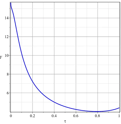
Figure 3 gives pollution in function of time from equation (35). The curve is reverse U-shaped because the increasing returns to scales property of abatement holds. At the beginning of economic development, environmental degradation increases as time passes but when the economy is sufficiently advanced in the stages of growth, pollution
Figure 3: Pollution in function of time
Figure 4 graphs pollution in function of GDP per capita. Like the previous curve, it exhibits an inverse U-relationship since the increasing returns to scales property of abatement holds. We see that at the beginning of growth, environmental degradation augments with income. But when the country is sufficiently advanced in its economic
Figure 4: The environmental Kuznets curve
Now let us analyze how the EKC is affected by the tax rate. We notice in figure 5
that an increase of the tax rate from 40% to 48%, which correspond to 8 percentage points augmentation, causes the EKC to move downward. This occurs because a tax expansion raises the resources devoted to the abatement technology which in turn reduce the level of pollution. Thus the role of taxes is to shorten the period it will take the EKC to form. Consequently, taxes are an effective instrument of economic policy for the reduction
of pollution in the model. Hence instead of waiting passively for the EKC to happen, government can use taxes to allow what would occur in a distance future in a short amount of time. This result is clearly visible in figure 6 when we set taxes to the value that maximizes the growth rateτ∗ ≈ 0.79. In this figure it obviously appears that both
Figure 5: Effect of an increase of the tax rate
Figure 6: Effect of the optimal tax rate
We said earlier that the turning point of the EKC is sensitive to government taxes. We graph this property in figure 7. We see that the effect of taxes on the turning point
is nonlinear. From this relationship, we find a tax rate threshold ofτ∗≈ 0.79. The same
[image:22.595.193.402.374.585.2]augmenting taxes, it will in the long-run cause the turning point to increase. This last fact could generate an N-curve type relationship between pollution and income observed in some empirical studies. This is visible in figure 8 where we plot the EKC for three tax rate values 0.40,0.79 and 0.95. We notice that when taxes go from 0.40 to 0.79, the level, the turning point and the time it takes the EKC to form are reduced. But when taxes vary from 0.79 to 0.95, the level of the EKC is reduced but both the turning point and the time it takes the EKC to materialize are increased. Consequently this provides some explanations about the formation of an N-curve type EKC.
Figure 8: EKCs and turning points according to different tax rates
[image:24.595.193.401.540.746.2]Figure 9 compares the pollution level of the representative agent and the social planner. It appears that the pollution level of the social planner is less than that of the representative agent. The EKC for the social planner reaches its turning point and materializes itself entirely even before the EKC for the representative agent attains its turning point. This happens because the social planner enjoys higher growth, so he devotes more resources to abatement which in turn aided by the increasing returns to scales property reduce drastically the pollution level caused by high consumption.
Table 2 provides the economic welfare in function of the tax rate. We notice that the welfare in the economy augments as the income tax rate increases until this one reaches the valueτ∗≈79%, the marginal tax rate that maximize consumption growth rate. When
the tax rate is above this threshold, welfare starts to decrease. Hence the tax rate that maximizes the growth rate is also the one that optimize welfare in the economy.
Table 2: Economic Welfare in function of the tax rate
Tax rate 30% 40% 55% 79% 85% 90% 95%
Welfare 1025.81 1737.40 2771.13 3620.03 3548.00 3370.05 3071.90
Now we calculates the elasticities of the turning point with respect to the parameters of the model in table 3. We consider an increase of 9% of each parameter with respect to its initial value. We observe that θ and η have a strong negative impact on the turning point. In contrast φ has a small positive effect. But the influence of this last
parameter is strongly counterbalanced by that ofθandη, which make that in overall the turning point decrease with respect to all these parameters and confirming the increasing return to scales property of abatement. An augmentation of the elasticity of government investment in the production function also reduces the turning point. Increasing the share of government consumption with respect to productive government spending reduces the turning point. This happens because this induces an expansion of government investment which as stated previously transpire to lessen the turning point. A rise in transfers to the household and a positive technology shock expand the turning point. This occurs since these two actions increase consumption which intensifies pollution.
Table 3: Elasticities of the turning point with respect to the parameters
Parameter τ η υ α θ ψ A ρ φ
4
Conclusion
In recent years, the problems about the global climate change have made that the is-sue of sustainable development has gained growing concerns among individuals with numerous backgrounds in the world. Since the beginning of the 1990s, the environmen-tal Kuznets curve has become one of the most hot research topics among economists about sustainable development in general and, the relationship between economic de-velopment and the environment in particular. This paper fits in these studies on the EKC and theoretically shows how a dynamic environmental Kuznets curve can emerge by introducing pollution and abatement technology in a public spending model of en-dogenous economic growth. The results show that if the increasing returns to scales property of abatement holds, an EKC arises in our dynamic endogenous growth model. The numerical simulations highlights that the turning point of the EKC diminishes when taxes augment and are below some threshold. Above this threshold the turning point begins to increase given some clarifications for the possible presence of an N-shaped Kuznets curve. Furthermore, the simulations demonstrate that taxes reduce the level of environmental degradation by pulling down the EKC.
Although the results were illuminating, some extensions may well be made. We could include a human capital sector in the model to see if this can help reduce the pollution level. We may possibly also analyze the effect of a Pigovian tax (Pigouvian tax) for
the reduction of pollution and a Pigovian subsidy for the increase of productive public spending.
References
Andreoni, J. and Levinson, A.: 2001, The Simple Analytics of the Environmental Kuznets Curve,Journal of Public Economics80(2), 269–286.
Barro, R. J.: 1990, Government Spending in a Simple Model of Endogeneous Growth,
Journal of Political Economy98(5), 103–125.
Berrens, R., Bohara, A., Gawande, K. and Wang, P.: 1997, Testing the Inverted U-Hypothesis for U.S. Hazardous Waste: An Application of the Generalized Gamma Model,Economic Letters55, 435–440.
Brock, W. A. and Taylor, M. S.: 2004, The Green Solow Model,NBERWorking Paper No. 10557.
Dinda, S.: 2005, A Theoretical Basis for the Environmental Kuznets Curve, Ecological Economics53(3), 403–413.
Egli, H. and Steger, T. M.: 2007, A Dynamic Model of the Environmental Kuznets Curve: Turning Point and Public Policy,Environmental and Resource Economics36(1), 15–34.
Grossman, G. M.: 1995, Pollution and Growth: What do we Know?, in “The Economics of Sustainable Development”. Edited by Goldin I. and Winters L.A., Cambridge University Press.
Grossman, G. M. and Krueger, A. B.: 1991, Environmental Impacts of a North American Free Trade Agreement,NBERWorking Paper No. 3914.
Grossman, G. M. and Krueger, A. B.: 1993,Environmental Impacts of a North American Free Trade Agreement., in “The U.S.-Mexico Free Trade Agreement”. Edited by Garber, P.,
MIT Press, Cambridge.
Grossman, G. M. and Krueger, A. B.: 1995, Economic Growth and the Environment,
Quarterly Journal of Economics110(2), 253–377.
Halkos, G. E. and Tsionas, E. G.: 2001, Environmental Kuznets Curves: Bayesian Evidence From Switching Regime Models,Energy Economics23, 191–201.
John, A. and Pecchenino, R.: 1994, An Overlapping Generations Model of Growth and the Environment,Economic Journal104(427), 1393–1410.
Kijima, M., Nishide, K. and Ohyama, A.: 2011, EKC-type Transitions and Environmen-tal Policy under Pollutant Uncertainty and Cost Irreversibility,Journal of Economic Dynamics & Control35, 746–763.
Kuznets, S.: 1955, Economic Growth and Income Inequality,American Economic Review
45, 1–28.
Panayotou, T.: 1993, Empirical Tests and Policy Analysis of Environmental Degrada-tion at Different Stages of Economic Development, World Employment Programme
Research,Working Paper 238.
Roca, J. and Alc´antara, V.: 2001, Energy Intensity,CO2Emissions and the Environmental
Kuznets Curve. The Spanish Case,Energy Policy29, 553–556.
Selden, T. M. and Song, D.: 1994, Environmental Quality and Development: Is There a Kuznets Curve for Air Pollution?, Journal of Environmental Economics and Environ-mental Management27, 147–162.
Selden, T. M. and Song, D.: 1995, Neoclassical Growth, the J Curve for Abatement and the Inverted U Curve for Pollution,Journal of Environmental Economics and Management
29(2), 162–168.
Shafik, N. and Bandyopadhyay, S.: 1992, Economic Growth and Environmental Qual-ity: Time Series and Cross-Country Evidence, The World Bank, Washington DC. . Background Paper for the World Development Report 1992.
A
Growth Rate of the Variables at the Steady-State
Divide both sides of equation (12) byK(t).d dtK(t)
K(t) =
(υ τ−τ+1)AK(t)1−αGI(t)α
K(t) −
C(t)
K(t) −
E(t)
K(t) −δ (49) SubstitutingGI(t) andE(t) by their respective values and simplifying further yields:
d dtK(t)
K(t) =(υ τ−τ+1)AAZ
α−C(t)
K(t) −
θC(t)
ηK(t) −δ (50)
WhereAZ= 1+ψ Aτ(1−υ)
(−1+α)−1
. Some more algebraic manipulations give:
K(t) γK−(υ τ−τ+1)AAZα+δ= −1−θ
η
!
C(t) (51)
With γK =
d dtK(t)
K(t) . Taking the logarithm and derivative with respect to time of both
sides of this last equation, we get:
d dtK(t)
K(t) =
d dtC(t)
C(t) (52)
From equality (19) we obtain:
d dtE(t)
E(t) =
d dtC(t)
C(t) (53)
And finally, from the production function we have:
d dtY(t)
Y(t) =
d dtK(t)
K(t) (54)
Equations (52) to (54) allows us to say that at the steady-state all variables grow at the same rate. This demonstrates the equality we have in (32).
B
Private Investment Rate
PIVR= IV(t)
Y(t) =
K(t)
Y(t)
d dtK(t)
K(t) +δ
(55)
Replacing output and capital growth rate by their respective values, we find:
PIVR= 1
A d dtC(t)
C(t) +δ
1+ψ
Aτ(1−υ)
!−1α+α
−1 (56)
Substituting consumption growth rate in this last expression, we have:
PIVR= 1
A (υ τ
−τ+1)A(1−α) 1+ψ
Aτ(1−υ)
!−1α+α
−ρ
1+ψ
Aτ(1−υ)
!−1α+α
−1 (57)
We observe that this private investment rate depends on taxes. In we replace in the values of the calibrated parameters, we obtain:
PIVR=0.2001332733 (58)