Estimating sign dependent societal preferences for quality of life

Munich Personal RePEc Archive

Estimating sign-dependent societal

preferences for quality of life

Attema, Arthur and Brouwer, Werner and l’Haridon, Olivier

and Pinto, Jose Luis

Erasmus University Rotterdam, University of Rennes, Glasgow

Caledonian University

2 September 2014

1

Estimating sign-dependent societal preferences for quality

of life

Arthur E. Attemaa_{, Werner B.F. Brouwer}b_{, Olivier l’Haridon}c_{, Jose Luis Pinto}d

a _{(Corresponding author) iBMG, Erasmus University, P.O. Box 1738, 3000 DR Rotterdam, the}

Netherlands. E-mail: [email protected], --31-10.408.91.29 (O); --31-10.408.90.81 (F) b _{iBMG, Erasmus University}

c _{CREM, Université de Rennes, France}

d _{Yunus Centre, Glasgow Caledonian University, UK.}

September, 2014

ABSTRACT. This paper is the first to apply prospect theory to societal health-related decision making. In particular, we allow for utility curvature, equity weighting, sign-dependence, and loss aversion in choices concerning quality of life of other people. We find substantial inequity aversion, both for gains and losses, which can be attributed to both diminishing marginal utility and differential weighting of better-off and worse-off. There are also clear framing effects, which violate expected utility. Moreover, we observe loss aversion,

indicating that respondents give more weight to one group’s loss than another group’s gain of

the same absolute magnitude. We also elicited some information on the effect of the age of the studied group. The amount of inequity aversion is to some extent influenced by the age of the considered patients. In particular, more inequity aversion is observed for gains of older people than gains of younger people.

Key Words: equity weighting, loss aversion, prospect theory, QALYs

JEL CLASSIFICATION:D63,I10

1 _{This research was made possible through a grant from The Netherlands Organization for Health Research and}

2

1. Introduction

Cost-effectiveness analyses are increasingly being used in health care policy in order to guide the allocation of health care resources. The concept of Quality Adjusted Life Years (QALYs) is an important tool to quantify the effects in these analyses. The major purpose of cost-effectiveness analyses is to obtain the highest health gains with a given budget. However, it is by now well-known that many individuals have a preference for the distribution of health gains alongside their magnitude (Dolan et al., 2005). In particular, people tend to give different weights to the same health improvements depending on severity (i.e., initial health status (Nord et al., 1999)), age (Johannesson and Johansson, 1997), lifetime health (Williams, 1997), and distribution among the population (Cuadras-Morató et al., 2001; Dolan and

Tsuchiya, 2011; Johannesson and Gerdtham, 1996; Lindholm and Rosén, 1998). These preferences reflect a trade-off between efficiency (defined as maximising health) and some other factor, which is likely to include equity considerations. Equity weighting is very

important for societal decisions and can have enormous ethical consequences. This highlights the need for incorporating equity weighting into health-related decision making, and to obtain proper empirical estimations of these weights.

3 Little research has been performed on equity weighting functions in the health

domain. Bleichrodt (1997) suggested the extension of rank-dependent utility theory from decision under risk to social decision making, by giving different weights to different

individuals or outcomes, in a similar fashion as assigning decision weights to probabilities in decisions under risk. Subsequently, Bleichrodt et al. (2004) pointed out that it may be

unnecessarily restrictive to model aversion to health inequality solely through a concave utility function, and showed that the rank-dependent approach is consistent with the most popular HRSWFs, including those used by Dolan (1998). Bleichrodt et al. (2005) were the first to apply this rank-dependent approach empirically by implementing an adaptation of the trade-off method (Wakker and Deneffe, 1996). They elicited the equity weighting function for quality-adjusted life years (QALYs) and reported inequity aversion, but they only

considered gains. Subsequently, Turpcu (2013) extended Bleichrodt et al.’s (2005) approach

to the loss domain, but did not elicit a loss aversion index. For gains, he found inequity neutrality for low proportions and inequity aversion for medium to large proportions. In the loss domain, there was inequity neutrality for all proportions.

The disadvantage of the approaches used by Bleichrodt et al. (2005) and Turpcu (2013) is that they are quite labour intensive, requiring several steps to elicit equity weights. In order to derive policy recommendations from research, it is common to obtain data from a sample that is representative for the general public. Using such a labour intensive approach in a large general public sample would be prohibitively expensive. Therefore, we implement a simpler and shorter method in an internet survey among a large, representative, sample.

Another interesting question to pursue is whether equity weighting, utility curvature, and loss aversion differ when the age of the group under consideration is varied. One reason why we might expect this is because reference points for health may vary with age. In

general, health deteriorates with age, so individuals may have diminishing expectations of the (average, normal or acceptable) health level of older people than that of younger people (Brouwer and van Exel, 2005; Brouwer et al., 2005). These lower expectations may translate into lower reference points for the elderly. In turn, downwardly shifting reference points may cause health levels that are perceived as losses for young people to become gains for elderly people. Furthermore, we know from cumulative prospect theory (CPT) that losses are generally treated differently than gains, with losses getting more weight than gains, and possibly different shapes of the utility functions for gains and losses and the equity weighting functions in both domains. Hence, even if individuals have the same utility and equity

4 different preferences for older people than for younger people because of a gain-loss

asymmetry. The amount of loss aversion may likewise also be age-dependent.

First, loss aversion predicts a particular quality of life (QoL) level to receive more weight for young people than for old, because this level is more likely to be a loss for the young than for the old. Second, if the utility and/or the equity weighting functions differ between gains and losses, a further difference in preferences for the separate age groups may emerge. For instance, individuals may be inequity seeking for a given prospect when it involves a young group, but nevertheless inequity averse for that same prospect when it involves an old group. A reason for such a difference is that people may be inequity seeking for losses and inequity averse for gains, in a similar fashion as is commonly found for monetary outcomes in a risk context (Kahneman and Tversky, 1979). There is no evidence yet to predict the effect of the utility/equity weighting difference on the differential

preferences for young and old.

As stressed by Bosworth et al. (2009), it is important to have qualitative information alongside quantitative estimates of preferences. Therefore, we also ask the respondents for explanations for choosing a particular option. To the best of our knowledge, our study is the

first to complement the elicitation of prospect theory’s parameters with arguments. This is

highly relevant, as it allows us to test whether the conclusions that are normally inferred from

specific parameter values, are indeed supported by respondents’ stated reasons for their

answers.

This research is the first to simultaneously elicit societal utility and equity weighting for both gains and losses, together with a loss aversion index in the quality of life domain. In addition, our research involves another difference to previous elicitations of the HRSWF. It can be viewed, in a way, as a combination of preferences for distribution and for age groups.

That is, our experiment estimates people’s societal utility function over QALYs alongside the

5 We find substantial inequity aversion2, both for gains and for losses. This can be explained by a concave utility function as well as by equity weighting of proportions. We also observe substantial loss aversion: losses for one part of the group loom larger than gains for another part. Some significant differences between different age groups are found, and the arguments provided by the respondents support the intuition attached to the parameters estimated on their responses to the allocation task.

The remainder of this paper is organized in the following way. Section 2 presents our model and introduces notation, Section 3 describes the experimental design, Section 4 gives the results and Section 5 provides a discussion and conclusion.

2. Method

2.1. Notation

We consider a population of n individuals of age L and let (q1, …, qn) denote the QoL

profile, giving QoL score q to individual i. Following Bleichrodt et al. (2005), we assume QoL profiles are rank-ordered with q1>…>qn, unless stated otherwise.

2.2. The CPT-QALY model

If we want to quantify the equity-efficiency trade-off, we have to obtain estimations of the parameters of the HRSWF. The general HRSWF may be written as W=f(q1,…,qn).

One frequently studied specification is the isoelastic function proposed by Wagstaff (1991). Dolan (1998) applied a two-individual variant of this function:

( ) ( ) (1)

Dolan (1998) then continues with discussing a special case of this function, the Cobb-Douglas function which is analogous to Eq.1.

In this paper, we employ the rank-dependent QALY model (Bleichrodt et al., 2004) and extend it to account for sign-dependence. We adopt two separate social utility functions,

6 one for gains and one for losses, two separate equity weighting functions, and include loss aversion. Moreover, we extend the rank-dependent QALY model to allow for nonlinear utility, as was also done by Bleichrodt et al. (2005). We thus end up with a social version of the individual QALY model under CPT (Bleichrodt and Miyamoto, 2003). We assume that the HRSWF represents the social value of the QoL profile (q1, …, qn) by:

∑ ( ) (2)

where the are equity weights, defined as _{( ) ( )}. The function is a

nondecreasing function defined over [0,1], with _{( )} and _{( )} .

The Cobb-Douglas function is compatible with the rank-dependent utility

representation (Eq. 2) if U(q) is logarithmic (Bleichrodt et al., 2004), with B conceptually similar to , In this paper, we elicit more general utility functions (power functions) and also perform a new test of the Cobb-Douglas HRSWF.3 Our model is more general than the Cobb-Douglas model of Dolan (1998), in that it allows for other parametric specifications for the individual utility functions than only power (e.g. exponential utility). Moreover, our model is more powerful than Eq. 1, because our weight parameter is much less restricted than B. Our model also allows for more than two arguments, although in this study we use only two arguments for convenience.

In the HRSWF, the ’s have a similar interpretation as in Bleichrodt et al. (2005):

they represent the equity weights attached to the proportion of the group obtaining the best [worst] outcome in the gains [losses] scenario. As explained by Bleichrodt et al. (2005, p.657), if is convex, then the policy maker is averse to inequalities, in the sense that he will always prefer a transfer of QoL from a group that has relatively high QoL to a group that has less, as long as the rank-ordering of the groups in terms of the QoL obtained is not affected. A weight lower than the amount of the proportion implies inequity aversion for gains, since the better-off receive less weight than the worse-off, and vice versa for losses. A concave shape of U(q) has a similar effect (i.e., favouring the worse-off), but for a different reason: additional QoL improvements have less value the better the quality gets.

Now, extending this model to include sign-dependence boils down to (Attema et al., 2013; Wakker, 2010):

3 _{Bleichrodt et al. (2005) found little evidence supporting it, but our study investigates it in a different setting}

7

∑ ( ) ∑ ( ) (3)

where QoL level is taken as a reference point. All QoL scores higher than are treated as gains, and all scores lower than are treated as losses.4

Loss aversion is an index defined as a currency unit expressing the rate of exchange between gains and losses. It is captured as follows (Shalev, 2002):

_{( ) {} ( )

( ) [ ( ) ( )] (4)

where u is a utility function defined on QoL. We use the power family defined by u(q) = qα for gains and u(q) = -(-q)β losses, with α,β>0. For α,β =0, u(q)=ln(q) and u(q)=-ln(-q), respectively. The power function is concave for gains if α<1, convex if α>1, and linear if α=1. For losses, it is concave if β>1, convex if β<1 and linear if β=1.Bleichrodt et al. (2005) indicated that their equity weighting function reflected both pure equity weighting and

‘insensitivity to group size’. These two concepts were distinguished by two separate

parameters. However, because we only elicit one point of the equity weighting curve, we are not able to make this distinction. We instead chose to use an unspecified population size (but we explicated that the groups were always of the same size).

Because eliciting both the full utility functions and the full equity weighting functions would cause too much of a cognitive burden to our sample, we implement another approach, based on the semi-parametric method proposed by Abdellaoui et al. (2008) and subsequently applied in a health context by Attema et al. (2013). We adapted the method by replacing the outcome unit by QoL as a percentage of full health. Furthermore, instead of eliciting the decision weight attached to one particular probability, in this case we elicit the equity weight attached to a particular proportion of a group of people.

2.3. Utility and equity weighting elicitation

4_{Because we only used two-outcome prospects in our experiment, prospect theory (Kahneman and Tversky,}

8 For each prospect j in the gain (loss) domain, we elicit a value _̅ such that the

respondent is indifferent between the entire group gaining (losing) _̅ percentage points of

QoL and the prospect that provides a higher amount (in absolute value) to half of the

group and a lower amount (in absolute value) to the other half. Value _̅ corresponds to a

constant allocation of health. In the gain domain, we have , in the loss domain,

. Assuming the respondent’s preferences can be represented by CPT and a power utility function, this indifference can be evaluated in the gain domain by the following equation:

̅ _{( ) (5)}

Solving this expression for _̅ gives us:

̅ ( ( ) ) (6)

The procedure is similar in the loss domain giving the following equation that enables the simultaneous estimation of the utility function parameter and the equity weight ω- _through

nonlinear least squares:

̅ ( (( ) ( ) ) ( ) ) (7)

2.4. Loss aversion elicitation

The loss aversion index λ could be estimated by selecting an improvement of quality of life above the reference point, and determining the loss below the reference point for which the subject was indifferent between a treatment giving a gain of to half of the group and a loss of to the other half, and the reference point . Based on the assumptions introduced in Section 2.3, this gives:

9 The mixed prospect, when solving for λ, results in the following value:

_{( )} (9)

To facilitate comparison with previous estimates of the loss aversion index, we also report

our loss aversion estimates in terms of the traditional approach, which is given by µ=λ+1.

3. Experiment

3.1. Subjects

A total of 517 subjects, representative for the Dutch general population, participated in the experiment.

3.2. Procedure

The experiment was conducted by a professional internet sampling company (Survey Sampling International). This company has much experience with internet surveys and a large representative database of subjects. The subjects were rewarded with a monetary amount to be given to a charity fund of their choice.

The experiment started with some questions regarding background characteristics. We gathered information about age, gender, number of children, marital status, income,

education, health status (as classified by EQ-5D-5L) and rating of health (according to a VAS).

Indifferences were elicited by a combination of choices and matching. We started with a bisection procedure that adjusted the value of q upwards or downwards depending on the chosen option. We used two of these choices to zoom in on an indifference point. Having narrowed down the answer range accordingly, we gave the residual range of possible

10 BOX 1. Illustration of the combined bisection/slider procedure

Iteration Treatment A Treatment B Choice

1 60 (40, 0.5; 80) A

2 50 (40, 0.5; 80) B

3 Slider from 50 to 60 (40, 0.5; 80) Move slider to 54

3.3. Stimuli

The experiment consisted of two different versions, with each respondent being allocated randomly to one of them. In both versions it was made clear to the subjects that they should imagine a group of similarly aged people having a particular QoL in terms of

percentages of full health. The QoL obviously cannot get higher than 100%, so this was the maximum of our outcome range. In order to prevent QoL from becoming extremely low, the minimum was set to 20%.

Version 1 (Unique Reference Point: URP) induced a reference point of 60% of full health, and proceeded by eliciting the utility function over both gains and losses as seen from this reference point yielding both gains and losses ranging between 0 and 40%. In the mixed prospect, again, a reference point of 60% was induced,. Since the reference point was the same for gains and losses in URP, we could also estimate a loss aversion index for this version.

11 degree of risk aversion when starting at 60% to the degree of risk aversion in the other two parts, and to estimate the amount of behavioral loss aversion.

The utility functions for both gains and losses were elicited by the use of 7 questions each. In the gain part, the subjects were given the opportunity to give the group one of two treatments that could improve their health status. The constant allocation option contained a treatment that would increase QoL with ̅ percentage points for the entire group, whereas the variable allocation option involved a treatment that would let half of the group gain

percentage points and the other half gain percentage points, with_{| | | ̅| |} | . All QoL values were contained in the interval [20%,100%]. We specified all QoL improvements to be transitional, lasting for 1 year. Subjects were told that afterward the health of the group members would (further) improve to full health. The reasons we chose a duration of the differential treatment effect of only 1 year were the following. First, it was essential that the duration was the same for all respondents, in order to guarantee homogeneity of stimuli among respondents. If we took remaining lifetime, this could be interpreted differently for different respondents and, hence, this would hamper comparability of the results. Second, a longer time span would decrease the survival probability during this span. Respondents may then accordingly reduce their valuation of the health improvement, which would again impose heterogeneity among respondents.

The instructions of the gain part told the subjects to imagine that, because of a disease, the health status of a group of L=50/60/70/805 year old people had deteriorated a while ago to a level of 20% of full health. However, recently, the doctors had discovered two new

treatments that could do something to combat the disease.

The health status of a group of L year old people would in the loss part deteriorate during the next year to a level of 20% of full health because of a disease. After that year, the disease would disappear naturally, and their health would return to 100%. However, two treatments were also available to reduce the loss encountered during the coming year. A translation of the full instructions is available in Appendix A.

One treatment involved a gain [loss] for the entire group. The other treatment was risky, giving a larger gain [loss] for half of the group, but a smaller gain [loss] (or none at all) for the other half of the group. The amount of the gain [loss] in the riskless treatment was then elicited such that the respondent was indifferent between the two treatments.

12 A mixed prospect was included to allow for estimation of the loss aversion

coefficient. The subjects were instructed to consider a group of L year old people whose health had deteriorated recently to a level of 60% of full health due to unknown causes. The disease would be cured by itself in one year, causing their health to return to 100%, but now also a treatment has become available that may improve these people’s health immediately. However, the effects of this treatment are uncertain, because for half of the patients it

generates serious side-effects, reducing their health even further, to a level of q<60%. For the other half of the group, the treatment has no side-effects and their health immediately

improves to 80%.

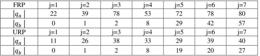
The stimuli of the prospects of these questions are shown in Table 1.

<TABLE 1 HERE>

Table 1. Stimuli of the gain and loss prospects for FRP and URP (in terms of absolute value of changes)

FRP j=1 j=2 j=3 j=4 j=5 j=6 j=7

| | 22 39 78 53 72 78 80

| | 0 1 2 8 29 42 57

URP j=1 j=2 j=3 j=4 j=5 j=6 j=7

| | 11 26 38 33 29 39 40

| | 0 1 2 8 19 20 27

We only used a proportion of one-half for the risky treatment. The order of the seven

prospects was random. The experiment always started with the gain part. After that, the loss and mixed prospects were asked in random order, although these parts were not interspersed. The latter would require more cognitive effort by the subjects, because they would then repeatedly have to change perspective from gains to losses, and vice versa, which would likely threaten data reliability.

Since we did not know the respondents’ reference points, we induced a status quo (i.e. an initial health state) that was the same for all. It may be the case that respondents adopted the status quo as their reference points, but they may also have framed the outcomes as

13 possibilities may evoke differences between them. Therefore, a significant difference

between age groups would reject the hypothesis that respondents perceive the status quo as their reference point, but instead replace or combine it with some other, age-dependent, reference point. In our experiment we also made an attempt to elicit this point by asking the respondents for normal health levels for people of several ages, as further explained below.

3.4.Explanations

We selected one choice in each part that was followed by a question about the reason why this particular option was chosen. In the gain part, we asked respondents who valued the equal prospect in the first choice of j=1 over the unequal prospect did so because of an equity heuristic, because of diminishing marginal utility6, or some other reason. Likewise,

respondents opting for the unequal prospect could choose between an argument of giving one part of the group a worthwhile improvement, an argument of increasing marginal utility, and some other argument.

Respondents choosing the equal allocation in the first choice of j=7 of the loss part could indicate a reason of inequity aversion (convex equity function), concave utility, or another or no specific reason. Those choosing the unequal allocation could opt for the argument of ensuring at least part of the group would keep its current health level (concave equity), convex utility, or again another or no specific reason.

For the mixed prospect we offered an argument of utility curvature or steepness (i.e., loss aversion) to the people not choosing the treatment in the first choice, as well as an argument of fairness, and again the possibility to give other arguments or having none. Finally, those picking the treatment had the opportunity to indicate an argument of ensuring at least one part of the group would experience a health improvement, an argument of utility curvature or steepness (i.e., gain seeking), or some other or no particular argument. The exact framing of the questions can be found in Appendix B.

3.5.Subjective health expectations

After the main experiment, we elicited the respondent’s perceived normal health level

at different ages. The latter was accomplished by using the EQ-5D-5L classification system

6 _{As shown in Appendix B, this means the respondents value a gain of 20 to 31 more than a further}

14 and asking for each of its 5 dimensions, at what age respondents thought it was normal to experience deteriorations, and to what degree (using the 5 levels of the EQ-5D, varying between no problems to severe problems). This question was being repeated for the ages 40, 50, 60, 70, 80 and 90 years. Respondents could also indicate they considered problems on some dimension never to be normal. The answers enabled us to compute for each age which EQ-5D-5L state was considered normal. Furthermore, by applying the Dutch national tariff set for EQ-5D-5L states (www.euroqol.org), we could assign a QoL score to these states. As explained later, this was used as an approximation of respondents’ subjective reference

points.

3.6.Analysis

A subject was classified as inequity averse [inequity seeking] if at least 5 out of 7 questions produced an inequity averse [seeking] answer (i.e., a _̅ lower [higher] than the expected value of the treatment). This allowed taking into account response error. Box 2 exemplifies this classification for the beneath answers of a virtual respondent.

Box 2. Example of classification

Prospect Treatment B EV _̅ Classification Atkinson

Index

1 (22, 0.5; 0) 11 10 Inequity averse 0.091

2 (39, 0.5; 1) 20 15 Inequity averse 0.250

3 (78, 0.5; 2) 40 30 Inequity averse 0.250

4 (53, 0.5; 8) 30.5 35 Inequity seeking -0.148

5 (72, 0.5; 29) 50.5 52 Inequity seeking -0.030

6 (78, 0.5; 42) 60 50 Inequity averse 0.167

7 (80, 0.5; 57) 68.5 64 Inequity averse 0.066

15 Because the data were not normally distributed (Kolmogorov Smirnov test: p<0.01 for

all _̅ ), we performed nonparametric statistical tests (Wilcoxon signed ranks tests for within-subjects analyses and Mann-Whitney tests for between-within-subjects analyses). The distribution of

̅ values was reasonably symmetric, so it was not necessary to first transform them. Two-tailed p-values are reported.

A convenient index can be derived from the HRSW function that provides a measure of inequity aversion: the Atkinson index (Atkinson, 1970). For gains, this is simply 1 minus the ratio of _̅ to the expected value (EV) of each prospect: 1- _̅ /EV (see also Dolan and

Robinson, 2001). For losses, it is ̅ /EV-1. Therefore, we also present the Atkinson indices as a summary measure of the amount of inequity aversion (also included in Box 2).

4. Results

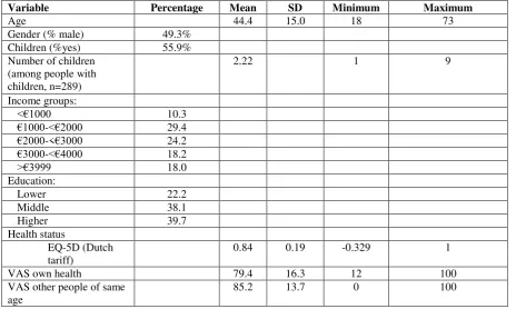
Table 2 shows an overview of the demographic variables for the entire sample of 517 respondents, which consisted of n=264 in FRP and n=253 in URP.

<TABLE 2 HERE>

Table 2. Background statistics (full sample, n=517)

Variable Percentage Mean SD Minimum Maximum

Age 44.4 15.0 18 73

Gender (% male) 49.3% Children (%yes) 55.9% Number of children

(among people with children, n=289)

2.22 1 9

Income groups:

<€1000 10.3

€1000-<€2000 29.4

€2000-<€3000 24.2

€3000-<€4000 18.2

>€3999 18.0

Education:

Lower 22.2

Middle 38.1 Higher 39.7 Health status

EQ-5D (Dutch tariff)

0.84 0.19 -0.329 1

VAS own health 79.4 16.3 12 100 VAS other people of same

16

Completion time (mins.) 24.1 10.6 5.9 80

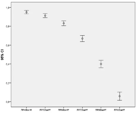
The data regarding expected normal health states for different age classes indicate a steep decline in the amount of health the higher the age (Figure 1). The average expected QoL declines from 0.94 for 40-year olds to 0.08 for 90-year olds. Most strikingly, respondents expect people of ages 80 and above to live in poor health states. For 90-year olds, the median expected health state was as low as EQ-5D-5L state 55553, which is lowest on four of the domains and is assigned a negative QoL value according to the Dutch tariff (EuroQol Group, 2013). These patterns clearly resemble previous findings in this area (Brouwer and van Exel, 2005; Péntek et al., 2012).

<FIGURE 1>

17 4.1CAEs and inequity attitude

FRP

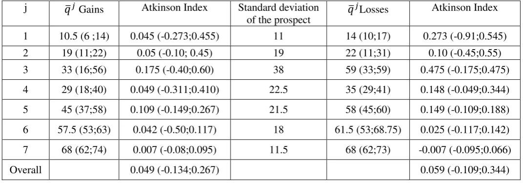
Table 3 displays the medians of the _̅ as well as their corresponding Atkinson indices for each prospect.

<TABLE 3>

Table 3. Median ̅ s (interquartile ranges)

j _{̅ Gains} Atkinson Index Standard deviation

of the prospect ̅ Losses

Atkinson Index

1 10.5 (6 ;14) 0.045 (-0.273;0.455) 11 14 (10;17) 0.273 (-0.91;0.545)

2 19 (11;22) 0.05 (-0.10; 0.45) 19 22 (11;31) 0.10 (-0.45;0.55)

3 33 (16;56) 0.175 (-0.40;0.60) 38 59 (33;59) 0.475 (-0.175;0.475)

4 29 (18;40) 0.049 (-0.311;0.410) 22.5 35 (29;41) 0.148 (-0.049;0.344)

5 45 (37;58) 0.109 (-0.149;0.267) 21.5 58 (45;60) 0.149 (-0.109;0.188)

6 57.5 (53;63) 0.042 (-0.50;0.117) 18 61.5 (53;68.75) 0.025 (-0.117;0.142)

7 68 (62;74) 0.007 (-0.08;0.095) 11.5 68 (62;73) -0.007 (-0.095;0.066)

Overall 0.049 (-0.134;0.267) 0.059 (-0.109;0.344)

For gains, 56.9% [37.2%, 5.9%] of the answers were consistent with inequity

aversion [inequity seeking, inequity neutrality]. Similar proportions were observed for losses: 56.3% [38.7%, 4.9%] of the answers reflected inequity aversion [inequity seeking, inequity neutrality].

18 <TABLE 4a>

Table 4a. Classification according to ̅ (FRP)

Losses Inequity averse Inequity neutral Inequity

seeking Mixed Total

Mean AI Gains Inequity

averse 74 0 11 37 122

0.24

Inequity

neutral 0 0 0 0 0

-0.01

Inequity

seeking 7 0 33 16 56

-0.31

Mixed 31 0 15 40 86 0.04

Total 112 0 59 93 264

Mean AI 0.30 -0.23 0.06 0.10

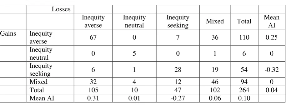
Since subjects were only classified as inequity neutral if they provided the EV as their CAE in at least 5 of the 7 questions using the above criterion, we also classified subjects using a criterion which allowed for a higher response error. In particular, this criterion also classified subjects as inequity neutral if they had a CAE that was within +/-2.5% of the EV at least five times. As shown in Table 4b, the classifications are quite robust to allowance for error.7

<TABLE 4b>

Table 4b. Classification according to ̅ when including an error margin for inequity

neutrality (FRP) Losses Inequity averse Inequity neutral Inequity

seeking Mixed Total

Mean AI Gains Inequity

averse 67 0 7 36 110 0.25

Inequity

neutral 0 5 0 1 6 0

Inequity

seeking 6 1 28 19 54 -0.32

Mixed 32 4 12 46 94 0

Total 105 10 47 102 264 0.04

Mean AI 0.31 0.01 -0.27 0.06 0.10

7 _{We also classified subjects using a 5% upper and lower margin (see Appendix C for results). This mainly}

19 Stochastic dominance, defined by the assignment of a higher indifference value to a prospect with at least one better outcome and no worse outcome, was also sometimes

violated. A significant minority of our subjects violated dominance in one or more questions, in that their indifference value was equal to the lowest or highest outcome of the prospect. This held for 5.25% of the CAEs in the gain domain and 7.31% in the loss domain.

URP

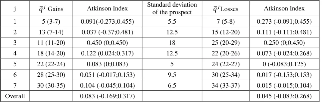
Table 5 displays the medians of the _̅ as well as their corresponding Atkinson indices for each prospect.

<TABLE 5>

Table 5. Median ̅ (interquartile ranges)

j _̅ Gains Atkinson Index Standard deviation _{of the prospect ̅} Losses Atkinson Index

1 5 (3-7) 0.091(-0.273;0.455) 5.5 7 (5-8) 0.273 (-0.091;0.455)

2 13 (7-14) 0.037 (-0.37;0.481) 12.5 15 (12-20) 0.111 (-0.111;0.481)

3 11 (11-20) 0.450 (0;0.450) 18 25 (20-29) 0.250 (0;0.450)

4 18 (14-20) 0.122 (0.024;0.317) 12.5 22 (20-26) 0.073 (-0.024;0.268)

5 22 (22-24) 0.083 (0;0.083) 5 24 (22-27) 0 (-0.083;0.125)

6 28 (25-30) 0.051 (-0.017;0.153) 9.5 30 (25-34) 0.017 (-0.153;0.153)

7 30 (30-35) 0.104 (-0.045;0.104) 6.5 34 (33-37) 0.015 (-0.015;0.104)

Overall 0.083 (-0.169;0.317) 0.045 (-0.083;0.268)

For gains, 66.2% [28.2%, 5.6%] of the answers were consistent with inequity aversion [inequity seeking, inequity neutrality]. The higher amount of inequity aversion for URP than for FRP was not to be expected, because of the smaller range in case of URP, but it was nevertheless significant (Mann-Whitney test comparing total amounts of inequity averse responses per subject, p<0.01).

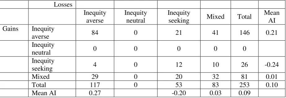
20 The classification of subjects in terms of inequity attitude for gains and losses is presented in Table 6a, and shows a similar picture as the one derived from the separate responses. The largest group consisted of subjects who were inequity averse over the whole domain (31.8%). There were also relatively many subjects who were inequity averse for either gains or losses and not classified for the other domain (15.5% for gains and 11.0% for losses). 12.1% could not be classified for both domains. Only 4.5% were classified as inequity seeking for both gains and losses. The proportion of universally inequity averse subjects was significantly higher than the proportion of inequity seeking subjects (binomial test, p<0.01).

<TABLE 6a>

Table 6a. Classification according to ̅ (URP)

Losses Inequity averse Inequity neutral Inequity

seeking Mixed Total

Mean AI Gains Inequity

averse 84 0 21 41 146 0.21

Inequity

neutral 0 0 0 0 0

Inequity

seeking 4 0 12 10 26 -0.24

Mixed 29 0 20 32 81 0.01

Total 117 0 53 83 253 0.10

Mean AI 0.27 -0.20 0.03 0.09

An alternative classification accounting for error (+/-2.5% margin) by inequity neutral subjects was also performed for URP and again gave similar results as in the initial

classification, as demonstrated by Table 6b.

<TABLE 6b>

Table 6b. Classification according to ̅ when including an error margin for inequity

neutrality (URP) Losses Inequity averse Inequity neutral Inequity

seeking Mixed Total

Mean AI Gains Inequity

averse 69 2 15 41 128 0.22

21 neutral

Inequity

seeking 2 0 7 10 19 -0.26

Mixed 29 5 10 60 104 0.02

Total 100 7 32 114 253 0.10

Mean AI 0.29 0.01 -0.27 0.02 0.09

There are also significant differences in the Atkinson indices of low and high outcome prospects. In particular, respondents were more inequity averse for lower gain prospects than for higher gain prospects. Vice versa, respondents were less inequity averse for higher loss prospects than for lower loss prospects. We found evidence for such effects both in FRP and in URP.

Stochastic dominance was violated for 3.78% of the CAEs in the gain domain and 8.13% in the loss domain.

Comparing gains and losses

We compared the _̅ in terms of final values between gain and loss prospects offering similar final values in FRP. For example, we compared prospect j=1 with the lowest gain to prospect j=7 with the highest loss, and vice versa. We also compared j=2 and j=6, j=4 and j=5, and j=3 with itself. We found significantly lower values for losses than gains for 5 out of the 7 comparisons (p<0.05). Lower values for losses corresponded to the five prospects with the lowest expected values. We also compared the Atkinson indices between these prospects. In these comparisons we again find more inequity aversion for losses than for gains for 5 out of the 7 comparisons (Wilcoxon signed ranks test, p<0.05), but also more inequity aversion for gains for the other 2 comparisons (p<0.01 for j=1 for gains vs. j=7 for losses, and for j=2 for gains vs. j=6 for losses).

For URP, the final health levels were different by design, so here we compared the Atkinson indices of prospects with the same absolute changes (e.g. j=1 with itself and so on). We found lower Atkinson indices for losses than for gains for 3 of the 7 comparisons

(p<0.05), and a higher index for losses for 1 (p<0.01).

Reference points effects within gains/losses

22 test, p<0.01) with URP associated with more inequity aversion. For losses, with final

outcomes 22 and 58, we found more inequity aversion for FRP (p<0.01). In both cases, we found evidence for a reference point effect: respondents were more inequity averse for the same outcomes when their initial health state was higher.

Mixed prospect (FRP and URP combined)

There was also a high degree of inequity aversion in the mixed prospects. In total, 68.7% of the responses were inequity averse, 20.3% were inequity seeking, and 11.0% were classified as inequity neutral. This degree of inequity aversion was comparable to the degree of risk aversion for mixed prospects found in previous studies eliciting loss aversion with monetary outcomes (Abdellaoui et al., 2008) or health outcomes (Attema et al., 2013).

4.2. Comparison of age groups

Mann-Whitney tests indicate a significant difference between the within-subject Atkinson indices of the sample with 50/60/70 year olds and the sample with 80-year olds. Atkinson indices differed between 70 and 80 years old for FRP in the gain domain and for URP in both domains, with higher inequity aversion for 80 years old people. We also found evidence (p<0.06) for inequity aversion between 50/60 and 80 years old for gains in FRP and losses in URP. People get more inequity averse when deciding on behalf of a group of 80 than on behalf of 50, 60 and 70 year olds.

4.3. Parametric estimates

Table 7 gives an overview of the parameter estimates when fitting the power family. The results make clear a considerable amount of concavity for both gains and losses, as well as a significant amount of equity weighting.

FRP

The power estimates α and β both indicate concavity, although the estimate only deviates significantly from 1 for losses (p=0.54 for gains; p<0.01 for losses). The estimates are significantly larger than 0, rejecting the Cobb-Douglas specification (p<0.01). The estimates of both ω+_{and ω}- _{are significantly smaller than 0.5 (p<0.01). We did not estimate}

23 URP

Both power estimates again indicate concavity, although it is not significantly different from 1 for gains (p=0.61 for gains; p<0.01 for losses). The Cobb-Douglas

specification is again rejected, with both estimates being significantly higher than 0 (p<0.01). The estimate of ω+ is substantially smaller than 0.5 (p<0.01), suggesting most of the inequity aversion for gains can be attributed to differential weighting of the two groups in this version. For losses the results are similar to those of FRP, with the estimate of ω- _{not significantly}

different from 0.5 (p=0.06).

The estimate of λ indicates loss aversion (p<0.01). However, this estimate is an underestimation of the amount of loss aversion, because 49 subjects were excluded from this analysis as their answer to the mixed was prospect was L=0, implying infinite loss aversion. Including these respondents in the analysis, the median increases to 2.65. Finally, the last column shows the loss aversion index in its traditional form (µ=λ+1).

<TABLE 7>

Table 7a. Estimation results, based on individual data (FRP)

α ω+ _{β ω} - _λ

Median 0.88 0.42 1.38 0.48 --

IQR 0.40-1.50 0.24-0.59 0.73-3.05 0.18-0.63 --

Table 7b. Estimation results, based on individual data (URP)

α ω+ _{β ω} - _{λ µ=λ+1 Incl. infinite LA}

Median 0.98 0.37 1.16 0.48 0.44 1.44 2.65 3.65

IQR 0.62-1.38 0.25-0.53 0.95-2.36 0.29-0.68 -0.49-20.3 0.51-21.3 -0.35-28121 0.65-28122

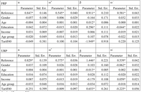
To account for the impact of socio-demographic variables, we also estimated a fixed-effect model taking account gender, age, education and income. We also included age groups and the tariff at 40. The latter allows accounting for the heterogeneity in perceived life quality. For gender, women were taken to be the reference. For age, we took the average age. For education and income we took the lowest level as a reference. For age groups, the

reference was the 50-years old group. For the tariff at 40, value 1 was taken to be the

24 on inequity aversion for losses in URP where both effects went in opposite direction. Here, men were found to be more inequity seeking for losses. The main effect of age was to increase the convexity of the utility function in both FRP and URP. Education had no effect in URP, but impacted both utility and weighting for losses in FRP, with higher education associated with more concavity in utility and less weighting. Both have opposite effects on inequity aversion. Finally, deviations from a value of 1 for the tariff at 40 mostly impacted the shape of the utility function in the loss domain in both versions, but we observed opposite signs here, which is difficult to interpret.

<TABLE 8>

Table 8. Fixed-effect regression on observable characteristics

FRP α ω+ β ω

-Parameter Std. Err. Parameter Std. Err. Parameter Std. Err. Parameter Std. Err. Reference 0.847* 0.146 0.545* 0.040 0.911* 0.210 0.581* 0.043 Gender -0.057 0.108 0.006 0.029 -0.164 0.171 0.032 0.033 Age -0.004 0.004 0.001 0.001 0.012* 0.006 0.000 0.001 Education 0.042 0.072 -0.015 0.020 0.296* 0.111 -0.044* 0.022 Income 0.031 0.069 -0.007 0.019 0.066 0.111 -0.019 0.021 Age group -0.020 0.049 -0.014 0.013 0.107 0.078 -0.022 0.015 Tariff40 -0.049 0.381 0.100 0.104 -1.949* 0.918 0.220 0.125

URP α ω+ β ω

Parameter Std. Err. Parameter Std. Err. Parameter Std. Err. Parameter Std. Err. Reference 0.829* 0.139 0.375* 0.036 1.446* 0.221 0.539* 0.042 Gender 0.037 0.109 0.026 0.028 0.103 0.160 -0.062* 0.032 Age 0.004 0.004 -0.001 0.001 -0.013* 0.005 0.002 0.001 Education 0.016 0.074 0.015 0.019 0.028 0.112 -0.020 0.022 Income 0.087 0.075 -0.015 0.019 -0.179 0.108 0.059* 0.021 Age group -0.033 0.048 0.016 0.012 -0.034 0.072 -0.018 0.014 Tariff40 -0.251 0.399 -0.009 0.097 0.653* 0.261 -0.225* 0.056

*: significant at 5%.

4.4. Explanations provided by respondents

Gains

25 instead of utility maximization. Indeed, this explanation is consistent with our empirical estimates, which indicate underweighting of the group gaining the most. The argumentative evidence therefore underlines the necessity to model this kind of preferences in terms of both a utility function and an equity function.

<TABLE 9>

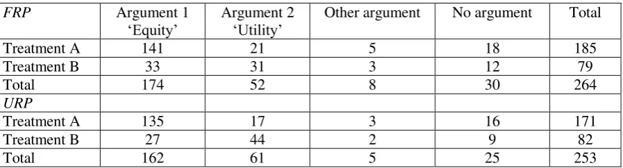
Table 9. Arguments for gain prospects

FRP Argument 1

‘Equity’ Argument 2 ‘Utility’ Other argument No argument Total

Treatment A 141 21 5 18 185

Treatment B 33 31 3 12 79

Total 174 52 8 30 264

URP

Treatment A 135 17 3 16 171

Treatment B 27 44 2 9 82

Total 162 61 5 25 253

For URP, the number of respondents choosing Treatment B in this question was less than half of the number of respondents choosing Treatment A. Among those, there was a majority stating Argument 2 (utility argument) as their reason for preferring Treatment B, although the difference was not as overwhelming as for the individuals picking Treatment A. However, the difference was significant according to a binomial test (p=0.028). This pattern suggests that there are more people choosing the unequal treatment do so because of a convex utility function than because of threshold reasoning, although for FRP, there was no

significant difference between the frequencies of the arguments (p=0.45).

We also compared the utility and equity weight estimates between the respondents choosing the different arguments, but these did not differ significantly (Mann-Whitney test, p>0.21).

Losses

26 <TABLE 10>

Table 10. Arguments for loss prospects

URP Argument 1

‘Equity’ Argument 2 ‘Utility’ Other argument No argument Total

Treatment A 62 118 0 20 200

Treatment B 31 9 1 12 53

Total 93 127 1 32 253

FRP

Treatment A 65 89 6 15 175

Treatment B 53 21 2 13 89

Total 118 110 8 28 264

For those choosing Treatment B, there was a majority stating Argument 1 (equity-related) as their argument (binomial test, p<0.01 for both versions). Hence, these people opted for the gamble in order for at least some people not to lose anything, which may be considered to be similar in spirit as the common observation where people prefer a monetary loss gamble over a sure loss if the former involves a chance of preventing a loss. A lower fraction of respondents indicated to have a convex utility function for losses, which would be consistent with Argument 2. In other words, people who prefer the risky treatment over the certain treatment tend to do so because of a reason that may be classified as giving more weight to the group of people with the best prospects after treatment (i.e., maintaining their present health status), rather than their utility function being convex. Again, this stresses the importance of separating these two concepts when modelling responses.

Mixed prospect

As indicated before, most people in the mixed prospect part were inequity averse, preferring to obtain the status quo over a treatment involving both gains and losses, with equal expected value of 0. However, within this group of respondents, arguments were equally divided between Argument 1 and Argument 2. Therefore, there was an equal split between people being inequity averse for reasons of fairness, and people being inequity averse because of utility curvature/loss aversion. This once again highlights the need for separating these effects when analysing and interpreting the data.

<TABLE 11>

27 Argument 1

‘Equity’ ‘Utility/loss aversion’Argument 2 argument Other No argument Total

No treatment 165 165 20 34 284

Treatment 74 34 2 23 133

Total 239 199 22 57 517

Finally, among the minority choosing the treatment, significantly more subjects indicated Argument 1 as their reason than Argument 2 (p<0.01). This suggests that, among the gain seeking respondents, most people give more weight to the group that can gain something, instead of having a convex utility function.

5. Discussion

The aims of this research were to extend the measurement of the HRSWF to losses, to estimate a loss aversion index, to test for possible differences between age groups, and to

obtain insight into people’s reasons for choosing particular options. Knowledge about the HRSWF is important to better understand inequity attitudes with respect to health and how these depend upon framing. Very little research has been done on this topic, with some notable exceptions (Bleichrodt et al., 2005; Turpcu, 2013). This paper has contributed to the literature in that it was the first to measure a loss aversion index in this context, which may, in addition to its frequently reported presence in individual decisions, be of importance in a societal context as well.Our approach was also novel in that we studied QoL improvements and deteriorations instead of longer-lasting QALY profiles.

We observed substantial inequity aversion for gains as well as losses in our

experiment and showed it can largely be attributed to both diminishing marginal utility and

‘pure equity’ concerns (as reflected by significant equity weighting). The amount of inequity aversion is even larger for losses than for gains, which is largely due to concave utility, as there is no substantial inequity weighting for losses. We also observed the presence of loss aversion and significantly different results for the two versions, indicating clear reference point effects.

28 their decision than the utility curvature argument. However, still a substantial minority of the respondents considered the utility argument to be of greater importance, underscoring the necessity to consider both these concepts in modelling the efficiency-equity trade-off. Furthermore, the finding that equity weighting appears to be more influential than utility curvature does not warrant the latter concept to be irrelevant, as demonstrated by the results of our parametric estimation; it only suggests that equity arguments are apparently more important than diminishing marginal utility arguments in this context.

For losses, to the contrary, there was a clear majority opting for the utility argument to be their main reason to choose the constant allocation. Therefore, these results give another argument to model gains and losses separately, since this is evidence that a separate

measurement of equity weighting and utility curvature is not sufficient: a distinct estimation of equity weighting and utility has to be performed for gains and losses, because these concepts turn out to be sign-dependent. This is again supported by the parametric estimates, which showed a significant difference between the equity weights for gains and for losses. More specifically, the answers to the motivational questions predict a larger deviation of the equity weight from 0.5 for gains than for losses, which was indeed confirmed by our

estimates.

The comparison of the age groups gave mixed results. There was some indication of respondents being more inequity averse when deciding on behalf of 80-year old people than when deciding on behalf of younger people, but no significant differences were found for the other comparisons.

29 Another limitation was that our experiment always started with the gains part.

However, after extensive piloting we deliberately chose this approach instead of randomizing because the gain task was easier to understand for respondents and after performing this task they were more familiar with the situation, so that they were better able to answer the loss part.

An explanation for our finding of significant differences between gains and losses may be that people are sensitive to framing and take the induced starting value as their reference point. However, it may also be that people have their own reference points for different age groups, but mix it up with the starting point, taking some value in-between as their reference point in the experiment. More research with higher sample sizes would be needed to further test this. Finally, our usage of an internet experiment may have lowered reliability of the results. A significant minority of our subjects violated dominance in one or more questions, in that their indifference value was equal to the lowest or highest outcome of the prospect. It would therefore have been better to use personal interviews, but this would be prohibitively costly.

Our results show a lot of mixed subjects, especially if we account for error margins. In order to find out more about these subjects, we performed several additional analyses on them (see Appendix D)8. One important conclusion that can be drawn from these analyses is that mixed subjects have a mean Atkinson Index close to 0. This implies that, even though mixed subjects are clearly not inequity neutral, they may be treated as “as if neutral” subjects

for societal decision making purposes.

Notwithstanding these limitations, we found some interesting results. First, the finding that diminishing marginal utility and inequity aversion are both relevant contrasts to the results from Bleichrodt et al. (2005) where most inequity aversion seemed to emerge from a convex equity weighting function instead of a concave utility function, and to Turpcu (2013), who found most inequity aversion to be due to concave utility. For gains, the answers to the argumentative questions are more supportive of the conclusions reported by Bleichrodt et al. (2005) than the conclusions from Turpcu (2013). Hence, our results highlight the need for more research into these two concepts of inequity aversion, in order to obtain more robust evidence as to its determinants.

Our findings agree with those of Bleichrodt et al. (2005) and Turpcu (2013) in that we reject the Cobb-Douglas function, i.e. the log-linear utility function, indicating utility is not as

30 concave in our study as in the study of Dolan (1998). Instead, part of the inequity aversion has to be accommodated by the implementation of a separate equity weighting parameter. The observation of loss aversion in our societal setting adds to the robustness of the loss aversion phenomenon. Previous research on individual decision making under risk already reported loss aversion to be expandable from the monetary to the health field (Attema et al., 2013; Attema et al., 2014). Moreover, Polman (2012) found evidence for loss aversion using monetary outcomes when people have to decide on behalf of others, although to a smaller extent than when deciding for themselves. We add to this evidence by our findings of loss

aversion when deciding on behalf of other people’s health. A head-to-head comparison implementing health outcomes in both an individual and a societal environment is

recommended for future research in order to compare the amount of loss aversion in these environments.

In conclusion, this paper has proposed a sign-dependent measurement of preferences for equity in health care and found this gain-loss distinction is indeed necessary. In particular, we reported that equity preferences are sign-dependent and can be attributed to both

diminishing marginal societal utility and lower weights being given to the worst-off. This was supported by arguments given by the respondents to justify their answers. Finally, loss

31

APPENDIX A. Translation of exemplary questions

Gains

We are about to ask you questions about what you would do in case you were a policy maker and had to make a choice between two treatments for patients on behalf of the Dutch

population. Because these are difficult questions and given that you probably don’t face this

problem in reality, we will first ask you some simple questions which will hopefully help you in answering this questionnaire.

We will speak about health as a number. If we say that the health of a group of people is 100, it means that the health of these people is perfect. If we say that their health is equally bad as being dead, then we give their health a value of 0. Can you indicate how you would rate your own health today on a scale from 0 to 100?

In the following questions, assume that the health of a group of 50-year old people has deteriorated seriously a few years ago. The cause was unknown and doctors could not do anything to improve their health. Their health is, expressed on scale from 0 to 100, only 20 now, while it used to be 100 in the past.

How would you appreciate a health of 20 on a scale from 0 to 100? -not very bad

32 Then now the good news. Doctors have found the cause of the problem. Not only that: two medical treatments are available. Both treatments ensure that the condition will completely resolve in one year, so that the health of this group of 50-year old people returns to the old level of 100. However, the treatments differ in the effect they have during the coming year. We will ask you to choose between these two treatments, but first we will better explain the choice problem using a stepwise procedure.

Question 1a.

The effects of Treatment A and B are indicated below. Which treatment would you choose now?

Health of the group 50-year olds without treatment: 20

Treatment A Treatment B





Losses

Practice question 1a.

Imagine a group of 50-year old people hasn’t felt very well the last time and goes to the

doctor. The doctor tells them they have a disease that causes their health to deteriorate to 10 during the next year. After this year, the disease is self-limiting and their health will return to the original level of 100. Two treatments are available that can reduce the consequences of the disease.

Treatment A causes the health of the entire group to drop by 45 from 100 to 55.

Health gain during next year Type I

patients

+22 (from 20 to 42) Type II

patients

0 (stays 20) Health gain

during next year Type I

patients (from 20 to 31) +11 Type II

patients

33 Treatment B causes full recovery in half of the patients (Type I patients): their health will

stay at 100. The treatment doesn’t work so well in the other half of the patients (Type II

patients) and their health immediately drops by 90: from 100 to 10.

Suppose you are a policy maker. You are not part of the patient group yourself and have to choose between the two treatments on behalf of the Dutch population. It is not possible to determine in advance who is Type I or Type II in Treatment B. This will only be resolved once the treatment has started. Moreover, you cannot choose Treatment B first and then A, or vice versa. You can choose only one treatment.

The initial health of the group and effects of the two treatments are summarized below. Can you indicate whether you would choose Treatment A or Treatment B?

Health of the group of 50-year olds before onset of the disease: 100

Treatment A Treatment B





Mixed prospect

Practice question 1a.

In the following questions, assume that the health of a group of 50-year old people has deteriorated seriously a few years ago. The cause was unknown and doctors could not do anything to improve their health. Their health is, expressed on scale from 0 to 100, only 60 now, while it used to be 100 in the past.

After one year, the disease is self-limiting and their health will return to the original level of 100. However, doctors have recently developed a treatment that may do something about the disease, but the effects of this treatment are uncertain. In exactly half of the group (Type I

Health loss during next year Type I

patients

0 (stays 100) Type II

patients

-90 (from 100 to 10) Health loss

during next year Type I

patients

-45 (from 100 to 55) Type II

patients

34 patients) the treatment works well. Those people immediately increase to a health level of 100 (a gain of 40). In the other half of the group (Type II patients) the treatment causes a lot of side-effects during the coming year. As a result, the health of those people immediately decreases to 40 (a loss of 30).

Suppose you are a policy maker. You are not part of the patient group yourself and have to choose between the two treatments on behalf of the Dutch population. It is not possible to determine in advance who is Type I or Type II in Treatment B. This will only be resolved once the treatment has started. Moreover, you cannot choose Treatment B first and then A, or vice versa. You can choose only one treatment.

The initial health of the group and effects of the two treatments are summarized below. Can you indicate whether you would choose Treatment A or Treatment B?

Health of the group 50-year olds before the disease: 60

No treatment Treatment





Health change during coming year

Type I

patients (from 60 to 100) +40 Type II

patients

-40 (from 60 to 20) Health change

during coming year

Type I

patients (stays 60) 0 Type II

35

APPENDIX B. Questions for explanations

Questions for arguments for choices

Arguments GAINS

If respondent chose the constant allocation in the first question of i=x, we asked the following question:

You indicated you would choose Treatment A. Did your choice have anything to do with one of the following reasons?

1. Both Types of patients will profit in that case. [EQUALITY/CONVEX EQUITY] 2. I consider an improvement from 20% to 31% more important than a further

improvement from 31% to 42%. [CONCAVE UTILITY] Response possibilities

Yes

Namely: Reason 1/2 No

I had another reason, namely:

I did not really have a reason for my choice

If respondent chose the unequal allocation in the first question of i=x, we asked the following question:

You indicated you would choose Treatment B. Did your choice have anything to do with one of the following reasons?

1. The people that won’t improve with Treatment B (Type II patients), are still in a

respectable health, so I would rather see a part of the group obtaining a substantial health improvement. [CONCAVE EQUITY]

2. I consider an improvement from 20% to 31% less valuable than a further improvement from 31% to 42%. [CONVEX UTILITY]

Response possibilities Yes

36 No

I had another reason, namely:

I did not really have a reason for my choice

Arguments LOSSES

If respondent chose the equal allocation in the first question of i=x, we asked the following question:

You indicated you would choose Treatment A. Did your choice have anything to do with one of the following reasons?

1. It’s not fair if the one part of the group loses more health than the other part.

[EQUALITY/CONVEX EQUITY]

2. I consider deterioration from 60% to 55% as less severe than a further deterioration from 55% to 49%. [CONCAVE UTILITY]

Response possibilities Yes

Namely: Reason 1/2 No

I had another reason, namely:

I did not really have a reason for my choice

If respondent chose the unequal allocation in the first question of j=1, we asked the following question:

You indicated you would choose Treatment B. Did your choice have anything to do with one of the following reasons?

1. Then at least 1 part of the group will keep the same health [CONCAVE EQUITY] 2. I consider deterioration from 60% to 55% more severe than a further deterioration

from 55% to 49%. [CONVEX UTILITY] Response possibilities

Yes

37 No

I had another reason, namely:

I did not really have a reason for my choice

Arguments MIXED PROSPECT

If respondent chose no treatment in the first question, we asked the following question:

You indicated you would not choose the treatment. Did your choice have anything to do with 1 of the following reasons?

1. It’s not fair if the one part of the group loses and the other part wins

[EQUALITY/CONVEX EQUITY]

2. A gain of 20 is insufficient to compensate for a loss of 20 [CONCAVE UTILITY FOR GAINS/CONVEX UTILITY FOR LOSSES AND/OR LOSS AVERSION] Response possibilities

Yes

Namely: Reason 1/2 No

I had another reason, namely:

I did not really have a reason for my choice

If respondent chose the treatment in the first question, we asked the following question: You indicated you would choose the treatment. Did your choice have anything to do with 1 of the following reasons?

1. Then at least a part of the group gets a better health [CONCAVE EQUITY] 2. A gain from 60% to 80% really makes a difference, while a deterioration from

60% to 40% does not make much of a difference [CONVEX UTILITY FOR GAINS/CONCAVE UTILITY FOR LOSSES AND/OR GAIN SEEKING] Response possibilities

Yes

Namely: Reason 1/2 No

I had another reason, namely:

38

APPENDIX C. Alternative classification of individuals

Table C1. Classification according to ̅ when including an error margin of +/- 5% for

inequity neutrality (FRP) Losses

Inequity averse

Inequity neutral

Inequity

seeking Mixed Total Gains Inequity

averse 48 0 4 35 87

Inequity

neutral 0 7 0 1 8

Inequity

seeking 4 1 24 16 45

Mixed 37 3 9 75 124

Total 89 11 37 127 264

Table C2. Classification according to ̅ when including an error margin of +/- 5% for

inequity neutrality (URP)

Losses

Inequity

averse Inequity neutral Inequity seeking Mixed Total Gains Inequity

averse 63 3 14 37 117

Inequity

neutral 3 2 3 10 18

Inequity

seeking 1 0 7 5 13

Mixed 26 6 7 66 105

39

APPENDIX D. Translation of exemplary questions

We performed a number of additional tests on the classifications as inequity

averse/neutral/seeking/mixed subjects both for gains and for losses. First, we computed the mean Atkinson index (AI) for each subject and compared the according classifications (i.e., averse [seeking, neutral] if AI>0 [<0, =0]) to the ordinal classifications that allow for an error margin of +/- 2.5% (Tables 4b and 6b). Ordinal inequity aversion [seeking] in almost all cases corresponded to a positive [negative] AI, and mixed subjects were about equally divided between positive and negative mean AIs.

Second, we computed whether this mean AI was significantly different from 0, and we found that for 95-100% of the mixed subjects this was not the case, whereas this percentage was below 40 for inequity averse and seeking subjects. Related to this, we calculated the mean AIs for mixed subjects with AI>0 and mixed subjects with AI<0 separately, and observed that the absolute values of these means were substantially lower than those of the non-mixed subjects.

Third, we computed the mean standard deviations for inequity averse subjects, inequity seeking subjects, mixed subjects with a positive AI and mixed subjects with a

negative AI. This gave very similar results, suggesting that mixed subjects were not classified as mixed because of being ‘confused’ or making more errors (which could be an explanation

40

References

-Abasolo I, Tsuchiya A. Exploring social welfare functions and violation of monotonicity: an example from inequalities in health. Journal of Health Economics 2004;23; 313-329.

-Abásolo I, Tsuchiya A. Is more health always better for society? Exploring public preferences that violate monotonicity. Theory and Decision 2013;74; 539-563.

-Abdellaoui M, Bleichrodt H, l'Haridon O. A tractable method to measure utility and loss aversion under prospect theory. Journal of Risk and Uncertainty 2008;36; 245-266.

-Andersson F, Lyttkens CH. Preferences for equity in health behind a veil of ignorance. Health Economics 1999;8; 369-378.

-Atkinson AB. On the measurement of inequality. Journal of Economic Theory 1970;2; 244-263.

-Attema AE, Brouwer WBF, l'Haridon O. Prospect theory in the health domain: A quantitative assessment. Journal of Health Economics 2013;32; 1057-1065.

-Attema AE, Brouwer WBF, l'Haridon O, Pinto-Prades J. An elicitation of utility over QALYs under prospect theory. Work in progress. 2014.

-Bleichrodt H, Diecidue E, Quiggin J. Equity weights in the allocation of health care: the rank-dependent QALY model. Journal of Health Economics 2004;23; 157-171.

-Bleichrodt H. Health utility indices and equity considerations. Journal of Health Economics 1997;16; 65-91.

-Bleichrodt H, Doctor J, Stolk E. A nonparametric elicitation of the equity-efficiency trade-off in cost-utility analysis. Journal of Health Economics 2005;24; 655-678.

-Bleichrodt H, Miyamoto J. A Characterization of Quality-Adjusted Life-Years Under Cumulative Prospect Theory. Mathematics of Operations Research 2003;28; 181-193.

-Bosworth R, Cameron TA, DeShazo JR. Demand for environmental policies to improve health: Evaluating community-level policy scenarios. Journal of Environmental Economics and Management 2009;57; 293-308.

-Brouwer WBF, van Exel NJA. Expectations regarding length and health related quality of life: Some empirical findings. Social Science & Medicine 2005;61; 1083-1094.

-Brouwer WBF, van Exel NJA, Stolk EA. Acceptability of less than perfect health states. Social Science & Medicine 2005;60; 237-246.