Development of a high power single mode laser for non linear optics applications
200
0
0
Full text
(2) DEVELOPMENT OF A HIGH POWER SINGLEMODE LASER FOR NON-LINEAR OPTICS APPLICATIONS by C.G. Sawyers Ph.D.. July 1981.
(3) UNIVERSITY OF SOUTHAMPTON. DEVELOPMENT OF A HIGH POWER SINGLE-MODE LASER FOR NON-LINEAR OPTICS APPLICATIONS. by. C.G. Sawyers. A thesis submitted for the degree of Doctor of Philosophy. Department of Electronics Faculty of Engineering and Applied Science. July 1981.
(4) UNIVERSITY OF SOUTHAMPTON ABSTRACT FACULTY OF ENGINEERING A N D APPLIED SCIENCE ELECTRONICS Doctor of Philosophy DEVELOPMENT OF A HIGH POWER SINGLE-MODE LASER FOR NON-LINEAR OPTICS APPLICATIONS by Craig George Sawyers. In the first part of this thesis an investigation is made into the feasibility of using a stable resonator which incorporates an intraeavity telescope as a means of extracting high power pulsed radiation in a TEMg. mode from a Nd:YAG laser.. An analysis of this telescopic. resonator is presented and experimental results are described.. TEM^g. mode operation has been verified with an output energy of 350mJ when the resonator was operated with a fixed Q, and lOOmJ when Q-switched. For many applications it is found that operation of the laser on a single-longitudinal cavity mode is desirable.. In the second part of. this thesis the conditions necessary to obtain single-frequency operation of a pulsed laser are discussed.. The application of one technique,. referred to in this thesis as pre-lase triggered Q-switching, has been investigated experimentally as applied to the telescopic resonator. Single-mode operation has been obtained for ^60% of laser shots, @nd guidelines are given as to how this fraction may be increased. The thesis is concluded by describing the application of the output from the telescopic resonator to two non-linear optical processes: frequency doubling and Raman scattering.. In each case it is shown that. with the laser operating single-frequency, good agreement is obtained between detailed theoretical prediction and experimental observation..
(5) CONTENTS Page. CHAPTER ONE:. INTRODUCTION. CHAPTER TWO:. TELESCOPIC RESONATORS FOR LARGE VOLUME TEM, 00 MODE OPERATION. 1. 2.1. Introduction. 4. 2.2. Theory of the Telescopic Resonator. 7. 2.2.1 2.2.2. 2.2.3. Preliminary remarks Derivation of an equivalent resonator for the telescopic resonator Choice of resonator parameters and telescope defocussing. 7 10. 23. 2.3. Choice of Mode-Selecting Aperture. 26. 2.4. Thermal Lensing of the Pockels Cell Q-SwiCch. 31. 2.5. Mode-Selecting Apertures: A Practical. 38. Point Concerning Their Design 2.6. Pockels Cell Alignment. 41. 2.7. Conclusion. 45. CHAPTER THREE: EXPERIMENTAL WORK ON THE TELESCOPIC RESONATOR. 47. 3.1. Introduction. 47. 3.2. Beam Spot-Size and Divergence. 47. Measurements: Method 3.3. CHAPTER FOUR:. Cavity Alignment Procedure. 54. 3.3.1. Telescope alignment. 54. 3.3.2. Resonator alignment. 55. 3.4. Tests on Practical Telescopic Resonators. 59. 3.5. Conclusion. 69. LINE NARROWING. 72. 4.1. Introduction and Review. 72. 4.1.1. 81. 4.2. A note on notation. Review of the Theory of Laser Linewidth. 81. 4.2.1. 88. 4.2.2 4.2.3. Fast Q-switching with no additional mode-selection Fast Q-switching with additional mode-selection Slow Q-switching with no additional mode-selection. 90 91.
(6) Page. 4.2.4 4.2.5. 4.3. 94. 102. 4.3.1. 103. 4.3.3 4.3.4. 4.3.5. CHAPTER FIVE:. 92. Practical Limitations and Their Effect on the Reliability and Pulse Repeatability of Slow Q-Switched Lasers. 4.3.2. 4.4. Slow Q-switching with additional raode-selection Mode-selection using Fabry-Perot etalons. The effect of random fluctuations in cavity length on mode-selection Transient and random cavity length changes Transient phase-shift induced by the Pockels cell Cavity mode pulling caused by dispersion in an intracavity etalon Cavity losses as a result of a tilted intracavity transmission etalon. 105 114 118. 121. Experimental. 122. 4.4.1 4.4.2. 123 127. The resonator Evaluation of performance. 4.5. Discuss ion and Recommendations for Further Work. 133. 4.6. Conclusions. 135. APPLICATIONS USING THE OUTPUT FROM THE TELESCOPIC RESONATOR: FREQUENCY DOUBLING A N D STIMULATED RAMAN SCATTERING. 137. 5.1. Introduction. 137. 5.2. Frequency Doubling. 137. 5.2.1. 137. 5.2.2 5.3. 142. Stimulated Raman Scattering of Frequency Doubled NdiYAG Radiation Using the Transition in Caesium Vapour. 149. 5.3.1 5.3.2. 149 152. 5.3.3. 5.3.4 5.4. Large signal energy conversion efficiency for harmonic generation using a singlefrequency pulsed laser Experimental results. General Calculation of the gain coefficient, g Estimate of the pump p o w e r necessary to reach Raman threshold Experimental. Conclusion. 154. 155 163.
(7) Page CHAPTER SIX:. CONCLUDING REMARKS. 164. APPENDIX 1:. Calculation of diffraction loss for TEM 00 and TEMj^Q modes. 165. APPENDIX 2:. Calculation of the number of resonator round trips of growth experienced by laser radiation during Q-switching. 168. APPENDIX 3:. Determination of the optimum face reflectivities for a single-plate resonant reflector used as a mode selector. 169. APPENDIX 4:. The relationship between the observed depth of modulation and ratio of mode powers for a laser operating on two longitudinal modes. 170. APPENDIX 5:. Large volume TEML_ mode operation of Nd:YAG lasers: Opt. C o m m : 37 (5), (1981), 359-362. 172. REFERENCES. 187. ACKNOWLEDGEMENTS. 193.
(8) CHAPTER ONE. INTRODUCTION. Since the invention of the laser over two decades ago, a large amount of work in resonator design has been directed towards achieving high power laser operation of pulsed lasers with a diffraction limited output beam, and good shot-to-shot repeatability. implies the need to work with a large mode volume.. In practice, this The work has been. motivated by the requirements of both industrial and scientific applications.. Industrial lasers used in a number of materials processing. applications (cutting, welding and drilling) need to have high output power and excellent long and short term stability (see, e.g. Steffen et al., 1972).. In the field of scientific applications the interpretation. and prediction of the behaviour in various laser interactions, e.g. n o n linear optical processes, can be significantly simplified if the laser provides a well defined spatial and temporal excitation.. For example,. most attempts at a theoretical description of non-linear optical processes assume incident laser beams to be Gaussian (Ward and New, 1969; Bjorklund, 1975; Cotter et al., 1975). Our own requirement for a high power, diffraction limited Nd:YAG laser arose from a preliminary investigation of stimulated Raman scattering in liquid nitrogen.. Published literature on this process had. suggested that the optical and material properties of liquid nitrogen were conducive to high efficiency Raman conversion (Grasyuk et al., 1977; Sinnott et al., 1977; Efimovskii et al., 1977; Grasiuk and Zubarev, 1978; Grasiuk, 1980; Grun et al., 1969).. Our first experiments, performed with. an unstable resonator Nd:YAG laser (Hanna and Laycock, 1979; Laycock, 1978) and a custom designed and built liquid nitrogen cell (Sawyers,1979), indicated that a major obstacle to the spatial quality of the Raman shifted (Stokes) beam was thermal blooming of the medium at laser repetition rates greater than. IHz (Wild and Maier, 1980; Smith, 1977;. Baklushina et al., 1977, Kormer et al., 1979).. However, even when the. repetition rate was reduced to the extent that thermal blooming was negligible, spatial distortion of the Stokes and transmitted pump was still observed.. Since the output beam from a diffraction coupled unstable. resonator is in the form of an annulus, it was not possible to make any accurate prediction of the expected Stokes beam profile.. Shortly. after these results had been obtained, a new Nd:YAG laser was purchased.
(9) from J.K. Lasers Ltd., under the tradename "Hyper Yag".. This involved. a new stable resonator design, incorporating an intracavity telescope (Sarkies, 1979).. This laser featured an output beam which had a much. smoother intensity profile than that of the unstable resonator, and in that respect was far superior for our applications.. Subsequent results. obtained using this laser to pump liquid nitrogen suggested that it w o u l d be desirable to operate the laser on a single-longitudinal mode.. At. first, an attempt was made to achieve this by applying to the Hyper Y a g laser a technique in which the laser incorporates frequency selection and the Q-switch is opened in two stages (Hanna et al., 1971; Hanna et al., 1972 (two papers)), known variously as two-step Q-switching, slow Q-switching, or, as we shall refer to it in this thesis, pre-lase Qswitching.. Disappointing results were obtained when this was applied to. the Hyper Yag, in that the reliability of single-mode operation was poor, and the transverse intensity profile of the beam showed shot-to-shot instability.. This led us to conclude that the Hyper Yag was operating. on several transverse modes, and that reliable and repeatable singlelongitudinal mode operation would only be secured when the laser operated on a single transverse mode.. We therefore embarked on a programme of. research aimed towards the operation of the Hyper Yag. (from now on. referred to as a telescopic resonator) with a single transverse TEM^^ mode and a single-longitudinal mode. Our first priority was to find out if the telescopic resonator was capable of supporting a large volume TEM^^ mode with good reliability. In the following investigations it was essential to have a detailed knowledge of the expected spot-sizes at various locations within the cavity.. Our early attempts at analysing the cavity in terms of ray-. matrices (Kogelnik, 1965; Kogelnik and Li, 1966) were frustrated by the unwieldy form of the results, and we consequently relied on numerical ray-matrix calculations using a digital computer (Clarke, 1980).. Using. these predictions as a guide, an appropriate aperture size and telescope magnification could be chosen to select a large volume TEJ^Q mode. Interactive use of the computer program and experimental w o r k led to a resonator design suitable for fixed-Q operation which produced an output energy of 350mJ in a diffraction limited beam.. Eventually, an analytical. approach was developed (Hanna et al., 1981 (two papers); M . A . Yuratich, Private Communication), providing simp1e, approximate design formulae which agree with exact calculations to the extent that the computer program has been dispensed with.. In Chapters Two and Three of this thesis.
(10) we present the analysis of the telescopic resonator and the experimental work performed to verify the single transverse mode behaviour of the laser, both when operated fixed-Q and Q-switched. In Chapter Four we consider the question of linewidth narrowing in pulsed lasers, and in particular the requirements for singlelongi tudinal mode operation.. One finds that the reliability and. repeatability of single-mode operation has an ultimate limitation, arising from changes in resonator length from shot to shot, and in the analysis of Chapter Four we derive an expression for the expected reliability of single-mode operation.. The chapter ends with a. description of the experimental results obtained for single-longitudinal mode operation of the telescopic Nd:YAG laser. We conclude the thesis in Chapter Five by describing the application of the output from the telescopic resonator to two nonlinear optical processes: frequency doubling and Raman scattering. Good agreement is obtained between theoretical prediction and experimental measurement for both these processes..
(11) CHAPTER TWO. TELESCOPIC RESONATORS FOR LARGE VOLUME T E M L . MODE OPERATION —— ^—-uU— —— ——. Sections 2.1, 2.2 and 2.3 of this chapter, and also Appendix 1, appear as submitted for publication to the Journal of Optical and Quantum Electronics.. Minor modifications, such as renumbering of. equations and figures, have been made to make its presentation compatible with the rest of this thesis. The final sections of this chapter are concerned with expanding on several points raised in sections 2.1 to 2,3, but which could not be elaborated on in the paper.. We also discuss some important practical. points arising as a result of the experimental work performed on the resonator, although detailed discussion of the experimental work is reserved for presentation as Chapter Three,. Abstract to the Paper A stable resonator incorporating a suitably adjusted telescope gives reliable operation of a Nd:YAG laser with a large volume. TEMQQ. mode.. The telescope adjustment is chosen to minimise. the effects of focal length variations in the laser rod and at the same time ensures the optimum mode-selection properties of a confocal resonator.. Simple approximations applied to the ray transfer matrices. allow a detailed analysis of the resonator to be performed.. This. analysis yields simple design equations relating the mode spot-sizes, resonator length, telescope magnification and defocussing, and diffraction losses.. Experimental results show excellent agreement with. the results of this analysis.. 2.1. Introduction By introducing a suitably adjusted telescope into a Q-switched. Nd:YAG laser resonator we have been able to obtain reliable operation with a large volume TEM^g mode (Hanna et al., 1981).. The basic. principle behind the resonator design is that of choosing a telescope adjustment which compensates the thermal lensing in the laser rod (thus permitting a large spot-size) and at the same time ensuring that the spot-size is insensitive to fluctuations in focal length of the.
(12) thermal lens.. In order to illustrate the principles of the design,. the discussion in the above paper was given in terms of a simplified resonator in which the telescope and laser rod were assumed short compared to the overall resonator length and located close to one mirror.. In fact, for accurate calculations in practical resonators. these assumptions are too restrictive and in this paper we derive the necessary design equations taking into account the finite length of resonator occupied by the laser rod and telescope.. However, before. introducing the resonator analysis we first briefly review some of the previous approaches to operation of NdzYAG lasers with high power and low beam divergence. It has long been appreciated that by compensating the thermal lens induced in solid state laser rods, one can increase the TEM^g mode spot-size and thus extract more energy in a diffraction-limited beam (Stickley, 1966).. However, it is found that in general this. compensation needs to be very precise if the mode size is to be comparable to typical laser rod diameters.. Fluctuations in the focal. length of this thermal lens (due to pump fluctuations) then lead to large spot-size fluctuations and thus unreliable performance of the laser.. Steffen, iWrtscher and Herziger (1972) pointed out this. important effect of focal length fluctuations but also showed that stable resonators could be designed which are insensitive to these fluctuations. resonators'.. They referred to these resonators as 'dynamic stable In one of their designs the resonator used two plane. mirrors with the laser rod close to one mirror and the mirrors spaced by half the focal length of the rod's thermal lens.. While this design. did permit reproducible operation of a NdzYAC laser with large volume TEM. mode, it suffered from an inconveniently long resonator.. Another design made use of a short radius convex mirror at one end of the resonator.. This produces a large spot-size at the other, concave,. resonator mirror (the laser rod is located here) and allows a conveniently short resonator to be used.. At about the same time. Chesler and Maydan (1972) also reported using a convex-concave resonator with a c.w. Nd:YAC laser.. In a later paper Lbrtscher et al. (1975). gave further details of the performance of their convex-concave resonator and their results amply confirm that it is possible to obtain reliable operation with a large volume TEM. mode. output was obtained from a pulsed NdzYAC laser).. (up to 850mJ fixed-Q However, the.
(13) disadvantage of the convex-concave resonator is that the spot-size is very small at the convex mirror and this effectively precludes its use in high power Q-switched lasers.. Thus Q-switched NdiYAG lasers. continued to be operated with conventional stable resonators which either result in a very multimode output when the full aperture of the laser rod is used or result in a small output energy when apertured down to give TEM^g operation. An important advance was made with the application of unstable resonator techniques to the Q-switched NdzYAG laser (Herbst et al., 1977) since this allowed the extraction of a large energy in a low divergence beam.. The advantages of this were immediately apparent in. such applications as harmonic generation.. However, the diffraction-. coupled output beam from an unstable resonator also has disadvantages associated with its non-uniform intensity profile.(Hanna and Laycock, 1979).. These shortcomings have stimulated a search for other means. (e.g. Brassart et al., 1977) of producing high output energy in a low divergence beam, but with a smooth intensity profile. reported using a telescope in a NdzYAG resonator.. Sarkies (1979). An attractive. feature of the telescope is that it allows easily controllable adjustment to compensate thermal lensing under varied pumping conditions. Although the output of his laser was not TEM^g, Sarkies found that a good working compromise could be achieved with high output power and low beam divergence.. We undertook our investigation of the telescopic. resonator with a view to gaining a fuller understanding of its behaviour and in particular of seeing whether a large volume TEM^^ mode could be obtained. In the course of our investigation we discovered that Steffen et al. (1972) had suggested a telescopic resonator configuration as one means of realising a dynamic stable resonator. In their publications they make no mention of having used a telescopic resonator and yet it offers two advantages over their convex—concave resonator.. These are (i) the easily controllable adjustment mentioned. above, and (ii) the fact that it avoids the very small spot on the resonator mirror, and can therefore allow operation at the power levels typical of a Q-switched NdzYAG laser.. There is a third attractive. feature, which applies to al1 dynamic stable resonators, namely that the diffraction losses produced by such resonators are the same as those of an equivalent symmetric which we derive in. Appendix 1,. resonator.. This result,. has not been referred to in earlier. discussions of dynamic stable resonators.. However, it has an important.
(14) bearing on the problem of TEM. mode selection since it is the confocal. geometry that provides the greatest degree of mode selectivity (Li, 1965).. This feature, and the two advantages referred to above, have. enabled us to obtain Q-switched. outputs of greater than lOOmJ. from a Nd:YAG laser with excellent reliability and without any damage problems.. 2.2. Theory of the Telescopic Resonator. 2.2.1. Preliminary remarks First we write down the standard result (Kogelnik and Li, 1966). for the Gaussian beam spot-sizes w^ and Wg at the mirrors 1 and 2 (curvatures R in figure 2.1.. and R^ respectively) of an empty resonator, as shown Expressed in terms of the g parameters, g^ = 1 - L/R^. and gg = 1 - L/Rg, we have. nw.. 2.1 'l^l. 8^82). J. and 'Wr. 2.2 82(1 - 8182). We shall be concerned, in the discussion that follows, w i t h resonators containing a laser medium which exhibits a thermally-induced lensing behaviour, having a focal length f^.. At first we shall assume the. laser medium to be adjacent to mirror 2, with the lens f^ incorporated in the curvature Rg.. It can be seen from equation 2.2 that the spot-. size, W g , in the laser medium can be made arbitrarily large by appropriate choice of R^, R^ and L. plane), then as gg ^ 1 so Wg. For example, with. = 1 (i.e. R^. In practice, however, such a choice. of parameters leads to a situation in which the spot-size Wg is extremely sensitive to the value of g^ and fluctuations in the value of fp^ will cause variations of w^ which are too great to permit reliable selection of the TEN. mode.. In fact, it can be shown from equation 2.2. that the fractional change, dwg/wg, of spot-size due to a fractional change, dgg/g^, is given by.
(15) 1-L/R. Figure_2il:. Empty resonator. 00.
(16) dw,. _. "2. 1 (28^82 - 1) dgg 4 (1 - 8182). 82. Thus as g^gg. 1 the spot-size Wg becomes sensitively dependent on g2. and hence. However, if one chooses g^g2 ° & then 2.3 shows that. spot-size Wg (but not w^) becomes insensitive to variations of This property was first exploited by Steffen et al.. (1972) in a. resonator having two plane mirrors, with the laser rod close to mirror 2 (thus g^ = 1, gg = 1 - L/fg), and the mirror separation, L, given by L = fg/2, hence ensuring g^gg =. Substitution of g^ = 1, gg = & in. equations 2.1 and 2.2 gives. 2.4. and w 2. =. 2 — IT. =. -is TT. 2.5. In this way, if f^ is large, then a large value of w ^ can be obtained (one can always introduce a lens to compensate the thermal lens thus making f^ effectively large).. The disadvantage of this approach,. however, is that the resonator is inconveniently long.. It is worth. noting here that this is actually a half-confocal resonator and an aperture placed at one mirror would therefore offer the ideal modeselectivity characteristic of a confocal resonator. (see Appendix I).. Another resonator design, which retains the condition g^g2 =. but allows a short length L, invoIves choosing mirror 1 to. be a very short radius convex mirror, i.e. making. >> 1.. -ve and. Thus g2 is also positive but gg. [R^l «. L, hence. 1, i.e.. corresponds to a concave reflector (R^ > 0) whose radius of curvature is slightly greater than L.. An examination of equations 2.1 and 2.2. shows that w ^ ^ = (g^/g^) « W g ^ and since g^gg =. 1. _ 2. this gives. 2.6. and 2 "2. _. 2AL 7T. 2.7.
(17) 10. Comparing equations 2.5 and 2.7 it can be seen that a large spot Wg can be produced in the laser medium (still assumed at mirror 2) with a short L provided. is large.. that this implies a very small w .. However, equation 2.6 shows. Thus although this resonator was. successfully demonstrated (Steffen et al., 1972; LBrtscher et al., 1975) for a fixed—Q Nd:YAG laser it would be unsuitable for a Q-switched laser. The telescopic resonator which we now describe provides a compromise between the two resonator designs given above.. To compare. its performance with these two resonators we anticipate the results of our analysis and quote here the expressions for w ^ and Wg, in the situation where (i) mirror 1 is plane, (ii) the telescope, of magnification M, is assumed short and is placed close to the rod, w h i c b itself is at mirror 2, and (iii) the telescope is adjusted to ensure insensitivity of spot-size w_ to variations of f . Z R shows that w^ and w^ are given by. w\2. Our analysis. =. — ir. 2.8. _. 1 LX ^ 2 2. 2.9. '1. and 2 *2. Thus, compared with the long resonator described by equations 2.4 and 2.5, for the same spot-size w^, the length of the telescopic resonator can be reduced by M^, although this makes w^ smaller by a factor M than the corresponding value in the long resonator.. On the other hand,. when the telescopic resonator is compared with a convex-concave resonator of the same length and same spot-size W g , then g^ in equation 2.7 takes the value. and it follows from equation 2.6 that the spot-. size w. in the telescopic resonator is M times larger than the spot-. size w. on the convex mirror.. 2.2.2. Derivation of an equivalent resonator for the telescopic resonator In making these preliminary remarks about the telescopic. resonator we chose a simplified resonator as an illustration.. In. practice, the simplifications made, such as assuming a short telescope.
(18) 11. and short laser rod, are too sweeping for accurate calculation.. We. now consider a telescopic resonator, shown in figure 2.2, for which the simplifying assumptions have been dropped.. Both mirrors are. assumed curved and the resonator contains a telescope of magnification M = -fg/f^ and a lens, focal length f^, representing the laser rod. The length L now refers to the length of that part of the resonator occupied by the contracted beam.. The telescope lenses are spaced by. d + 6 where d = f^ + fg and 6 is referred to as the telescope defocussing.^. The centre of the laser rod is spaced an optical. distance Gg from the telescope lens f2, and the m i r r o r Rg is spaced a further optical distance. from the rod centre.. We shall find it convenient to treat a mirror of curvature R as a plane mirror with an adjacent lens of focal length R in front of it.. This approach has the merit of allowing the resonator properties. to be calculated in terms of the single-pass ray-transfer matrix elements, where a single pass takes one from the left-hand plane mirror (plane 1) to the right-hand plane mirror (plane 2). The analysis is aimed at finding simplified expressions for the spot-sizes w. , w^ and in particular at finding the value of 6 which. makes Wg insensitive to variations of f^.. Our procedure is first to. consider the case where mirror 2 is in fact adjacent to the rod, and the rod is short, so. = 0, and where the rod is in the focal plane. of the telescope objective (lens f2) so. " ^2". This gives compact. and exact results which exhibit the main features of the telescopic resonator.. It is then possible to relax the above restrictions, and. introduce arbitrary spaces Agi &^' the formulae are more complex, and we discuss their approximations. It is readily shown that the ray matrix of the telescope f., d + 6, fr I S. M -. d + 6. 2.10 J. ^1^2. M. t Strictly, if the resonator length is to remain fixed as the telescope defocussing is varied, L should be replaced by L - 6. We shall ignore this small correction, however, as it can be shown that it has a negligible effect..
(19) L •2. f.. Mirror 1 Curvature Spotsize. f2. Telescope Spotsize W3. fp Laser rod. Mirror 2 Curvature R^ Spotsize W2 '. The telescopic resonator. N).
(20) 13. This matrix may be factorlsed telescope', a thin lens. 1. -^2. into a space. a 'thin. and a space -fgi. 1. 0. 0. M. 1. -^1 2.11. 0. 1. 2l. i. 0. 1. 0. 1. M. where the ray matrix of the thin telescope is. M. 2.12 0. -. M. and the thin lens' focal length is. 1. _. 6. f_. ". fo*. 2.13. The effect of the thin telescope is to expand the b e a m waist by a factor M and to reduce the beam curvature by a factor M, so that there is a beam discontinuity in its plane.. Note that the telescope. defocussing is described by a single element, the lens f . provides a key to the telescopic resonator.. Equation 2.11. It shows that the resonator. is exactly equivalent to one containing the following sequence of elements; a lens R , a space L', where. 2.14. L - f^. the thin telescope, a lens pair f , f space. and a lens R^.. separated by a space tg " ^2'. By choosing Kg ° fg, * the lenses f^ and f^ are. made adjacent and form a compound lens.. Since 1/f. is proportional to. 6, the compound lens has an adjustable focal length, which can be used to precisely compensate its rod lens component f . further restriction that length Rg, where. By making the. = 0, we have a compound lens of focal.
(21) 14. j_. ^. 2.15. 1^2. ^2. The restricted resonator with Kg " f2 figure 2.3.. ~ 0 is depicted in. Its eaxzat single-pass ray matrix is ——. A. B. ML. 2.16. =. (1 - G^Cg) C. D ML'. where the G parameters are given by. r M. 2.17(a). 1 Rn. r 1. M. -. M^L'. 2.17(b). Ro. With the help of these equations one can express spot-sizes in either of the commonly used ways, viz. in terms of A, B, C, D, or in terms of C^, C^.. The latter are particularly convenient for a. discussion of resonator stability.. The G parameters defined here are. a generalisation of the usual parameters g , gg for an empty resonator, and if we let M = 1, i.e. the telescope is removed, then G^. g^ = 1 - L/R^ and Gg. 82 " 1 - L/Rg.. As shown by Baues (1969) the spot-sizes are given by. 2.18(a) AC. TTWr, 2.18(b) CD. It is convenient to normalise the spot-sizes to & L. , bearing in mind. that typically L ' is approximately equal to the length L of resonator occupied by the contracted beam..
(22) L' _A_. fy fp R2. W'. W:. W'. Thin telescope. Figure_2i3:. Equivalent telescopic resonator with both thin telescope and laser rod located at mirror 2 Ul.
(23) 16. Thus the normalised spot-. 1 *w^2 W, 1. =. 2.19(a) XL'. 0^(1 - G^Gg). 1 M^G, 2.19(b). W. XL'. L ^2(1 - GiG,). L.. and at the entrance to the telescope, i.e. at the lens. the spot-. size IS. 2"^. W, 2.19(c). W, XL'. M. Figure 2.4 shows the behaviour of the spot-sizes W^, Wg, a function of. with G. and M fixed.. as. From equations 2.15 and 2.17,. these curves also represent the dependence of spot-sizes on telescope defocussing 6. figure.. A number of important results are indicated in this. First we note that the spot-size Wg is insensitive to. variations of. when G^ = 1/2G^, i.e. when G^Gg =. therefore the desired operating point.. and this is. In fact a comparison of. equations 2.19(b) with 2.2 is enough to show that the earlier condition ° i now becomes G^Gg = &.. The spot-sizes W ^ , Wg, W. for G^Gg = i. are indicated in figure 2.4 as /2MG^, /2G^/M and /M/G^ respectively. Thus the ratio of spot-sizes, Wg/W^, is G^/2, an important quantity to bear in mind when considering the question of damage to components in the contracted beam.. For the particular case w h e r e mirror 1 is plane,. G^ then has the value M and the normalised spot-sizes Wg, W ^ ,. are. /2M, /2 and 1 respectively, a result previously quoted in equations 2.8 and 2.9.. From figure 2.4 it can be seen that the minimum of #2 is. quite flat and from equation 2.19(b) one can show that a 10% change of Gg about the operating point G^Gg = & (i.e. Gg varying from 0.4/G^ to 0.6/CL) causes only a 1% increase in W_. vary and (dW^/dCg)^ ^. _ * =^MG^.. The spot-size W. does, however,. The figure also indicates that as. one approaches the boundaries of stable operation G^^^ = 1) the spot-size W. (at Gg " 0 and. diverges, whereas the spot-size. goes to.
(24) 17. Spot i. FiguTe_2^4:. Normalised spot-sizes fixed values of M and G,. , Wg,. versus Gg for.
(25) 18. zero as G2 ^ 0 and diverges as. ->-1.. In section 2.2.3 we discuss. the choice of & which optimises Gg and hence the performance of the telescopic resonator. The stability behaviour can be illustrated with reference to the G Gg plane, of which the positive quadrant is shown in figure 2.5. The stable region is enclosed by the G , G^ axes and the hyperbola G^Gg = 1.. The locus of ideal adjustment G^Gg = & is also a hyperbola,. passing essentially through the centre of the stable region. resonator with mirror 1 plane (G R2 > L (hence G. An empty. = 1) and mirror 2 concave with. > 0) is represented by a point on the line PQ.. The. point U represents the half confocal resonator, Q the plane-plane resonator.. If a thin telescope of magnification M is inserted adjacent. to mirror 2 in the resonators represented by the line PQ, they will then be represented by points on the line RS, w i t h the point S corresponding to the plane-plane resonator and the point V corresponding to the ideal operating point.. As the magnification M is increased, so. the range of values of Gg for stable operation is decreased. Having discussed the properties of the telescopic resonator with the particular choice arbitrary spacings.. = fg and 2^ = 0, w e now consider. Whereas the first case allowed us to derive exact. and compact expressions, in the case of arbitrary spacings the exact expressions are very cumbersome.. Exact results can, of course, be. obtained on a computer, but our aim here is to show that in fact the expressions derived above remain quite adequate for practical spacings. Any ray matrix can be put into the form o f equation 2.16, and with appropriate parameters G^, Gg, L ". say,. all the discussion. relating to figure 2.4 and equations 2.18 and 2.19 for the spot-sizes still applies.. However, the expressions for. , Gg, L'" (and hence. A, B, C, D) in terms of the physical resonator parameters will now differ from the G^, G^, L ' of equations 2.14, 2.17.. F r o m 2.18 it is seen. that the spot-sizes vary as B^, and so any small error in B will be insignificant.. On the other hand, the spot-sizes vary as 1/C* and l/D*,. and so errors in G or D will have a large effect on the spot-sizes, since the limits of the stable region are defined by C = 0 and D = 0. We conclude that when making approximations, C and D need more care than B; A can be regarded as a derived parameter since AD - EC = 1. Consider first the case where 2^ ^ f^. readily determined, and may be put into the form. The matrix elements are.
(26) 19. Locus of ideal adjustment, GiG2=1/2. /. -1 11 2M M 2 %^gure_2^5:. Stability diagram.. The line PQ represents stable empty. resonators with mirror 1 plane (G^ = 1). represents stable resonators with. The line RS. thin telescope. adjacent to mirror 2, and mirror 1 plane (G^ = M ).
(27) 20. V. 1 +. M /1. ML. 2.20(b). 1 +. 1 -. 2.20(a). ). R,. M^L'/l - —. ^ ML. A. /1 -. 1 - M. 1 _ ML'^I. 1. M. R.. /. i. M ^. M. Rr. 2.20(c). R:. 2.20(4). where. A. f. =. %2 - fg. 2.21(a). —. 2.21(b). fR. + 1_ *2. 1_ + _ J L R,. f?. 2.21(c). f - 6. In practice,. |A| «. or can be made so by design.. 2.22. |f|, |f^|, M^L'. Thus the term A/f can be dropped from. equation 2.20(d), giving. \ D. 1. /,. M^L'. M. 1. R. 2.23(a).
(28) 21. Note that the limit of the stable region defined by D = 0 is still an eaact function of. and hence of the defocussing 6.. Turning to. equation 2.20(c), then with Gg defined by equation 2.23(a) and by comparison with element C in equation 2.16 it is seen that a suitable choice of G^, and hence of A , is. A. =. =. M (1 - —. I. 2.23(b). ^1. As with D, this choice gives the zero of element C eazzotZy. approximated by dropping the terms 6/f. B. =. ML', L ". =. B can be. and A/M^L'(1 - A/f^), giving. L'. 2.23(c). (It is seen that we have effectively approximated A in the same way as B.). To summarise, we have found that by making the assumptions in. equation 2.22, then our earlier treatment of the telescopic resonator comes through with the one change, of IAI <<. to Rg .. Moreover, as. IfI from equation 2.22, then we can generally ignore the change,. and use the original equations 2.15 to 2.17. Figure 2.6(a) shows the actual resonator lenses f , their spacings A, special case A = just examined.. Rg and. Figures 2.6(b) and (c) respectively depict the = 0 treated earlier, and the case A ^ 0,. The last case we wish to examine, A = 0,. shown in figure 2.6(d).. = 0 f 0, is. By comparing with figure 2.6(c) it is apparent. that the expressions 2.20 can again be used, but w i t h the changes 1/f^ -+ 1/f^ + 1/fgy A. & , and 1/f. l/Rg.. corresponding to equation 2.22 are. <<. The inequalities. [Rgl, ll/f^ * l/fg^|. and which again are satisfied in practice.. wfl/,. Hence the only change from. the first expressions 2.15 to 2.17 is that R^ is replaced by where. -1*2. Again. =. + ^T. ^R. 1. 2.24. *2. can often be omitted, for example in the instance where mirror. 2 is plane. lengths, A =. However, whereas A is the difference of two comparable " fg, and so always tends to be small,. may give a.
(29) 22. T. T. R. 'R. fT. rt2. fp Rz (c). fy ^R. F^gure_2^6:. 2. Various cases of resonator lens combinations.
(30) 23. significant correction in equation 2.24, and hence to the predicted defocussing 6 in f^.. 2.2.3. Choice of resonator parameters and telescope defocussing In the previous section we have shown that the telescopic. resonator can be characterised by the values G^, resonator containing a thin telescope.. of its equivalent. We concluded that the telescopic. resonator should be adjusted so that its equivalent resonator satisfies the condition G^G2 =. This can be achieved by adjusting the telescope. defocussing 6, since this determines f (through equation 2.15) and finally. (through equation 2.13), hence (through equation 2.17(b)).. Thus with G^G2 put equal to & we find that 6^ ^ is given by. 1. opt. -. 1. M. %. 2Gi. /^1 - 2 R, 2.25 2M^/. V. 1 - ^ R,. fR. *2. Once the resonator parameters M, fg, L, R^, Rg have been chosen and fn is known, then 5 ^ can be calculated from equation 2.25. R opt ^ of f. The value. depends on the operating conditions (repetition rate and pump. energy) and provided its dependence is known, one can then calculate the necessary change of 6^ ^ for changed operating conditions. effect of a change in f^ is to change R^ and hence Gg.. This simply. translates the curves in figure 2.4 parallel to the G^ axis. of 6 has exactly the same effect since it changes f. The. A change. and hence Rg.. Thus the curves of figure 2.4 also indicate the dependence of spotsizes on telescope defocussing.. This behaviour provides an experimental. means of identifying whether one is operating at the optimum point.. As. is made to depart from its optimum value by changing the telescope defocussing it is found that the laser output energy drops and the beam quality degrades.. This drop in performance shows a symmetric behaviour. on either side of the optimum so that, for example, a plot of output energy versus 6 will exhibit a rather flat m a x i m u m and thus can be used to locate 6^ ^ roughly.. Fine adjustment of 6 ig usually then required.
(31) 24. for final optimisation of performance. We have indicated how 6 parameters are chosen.. . can be calculated once the resonator opt. We now consider some of the factors that. influence the choice of these parameters.. Obviously one cannot give. here an all-embracing strategy for the optimum selection of these parameters since they are influenced by the operating conditions of the laser.. For example, if the laser is Q-switched then it is likely that. damage limitations of components in the contracted beam will be a major factor in deciding the energy to be extracted. choice of spot diameter in the laser rod.. This influences the. Under fixed-Q conditions. quite different considerations apply and the maximum spot-size in the laser rod may then be determined by inhomogeneities caused by thermallyinduced birefringence (Koechner, 1976).. If damage is the main. limitation then one must seek a compromise between the convenience of a short resonator with its greater risk of damage and the inconvenience of a long resonator.. This choice can be illustrated most clearly by. considering a resonator with mirror 1 plane (G^ = M , and, since G G2 =. then. = 1/2M) for which equations 2.19(a) and 2.19(b) yield. 1. WgZ. =. =. k A TT. 2.26. AM' TT. 2.27. Equation 2.27 shows that for a given Wg, the smaller one makes choosing a larger M), the smaller is w^.. (by. This increases the risk of. damage due to the higher energy density and also, since the resonator is shorter, due to the shorter pulse duration.. The damage limitations. of dielectric coatings have led us to use an uncoated plane parallel plate of fused silica as the reflector for the contracted b e a m and this then serves as the output mirror. The laser used in our experiments has a 75mm x 9mm N d i Y A G rod pumped by twin flash-lamps.. We have operated this laser w i t h TEMg^ spot. diameters (2%^) up to 5mm and it is likely that at repetition rates of less than lOHz, where thermally-induced birefringence effects remain small (Koechner, 1976), even larger spot-sizes w o u l d be feasible.. A. typical set of resonator parameters that we have used for most of our work are as follows:- L = 0.34m, M = 4, f. =-0.05m (hence fg " 0.20m and.
(32) 25. d = 0.15m), &2 ^ 0.25m, & 2.14),. = 0.51m.. Hence L ' = 0.39m (from equation. = 0.36mm (from equation 2.26), Wg " 2.1 m m (from equation. 2.27).. The overall optical length of the resonator was 1.25m and. when the output energy E was ^lOOmJ the pulse duration T was measured to be 30ns (FWHM). then 2E/nw 1.6Cw/cm^.. The peak intensity at the resonant reflector is. = 2E/XTL', which for our parameters gave a value of This is to be compared with values for the damage threshold. of spectrosil B, when subjected to 10ns pulses of 1.06wm radiation, viz. 5Gw<6m^ (R. Wood, Private Communication).. The spot-size w ^ at the small. lens of the telescope is, according to equation 2.19(c), /2 greater than w^.. We have found that AR coatings on this lens are liable to. damage and an uncoated lens of BK7 is therefore used.. Apart from the. use of uncoated optics in the contracted beam we have not made any serious attempt to optimise the damage threshold.. Our laser has been. operated with the resonator parameters listed above, producing Q fi * -j switched outputs of ^lOOmJ for ^ 1 0 shots so far with no sign of damage. To optimise the damage threshold one would need to examine the various trade-offs, such as increasing the resonator length, decreasing the magnification, etc., and equations 2.19(a) and 2.19(b) provide the basis on which to carry out this optimisation analytically.. The. simplicity of the design equations 2.13 to 2.19 and 2.25 makes their use very straightforward. For the exact calculation of spot-sizes one needs to know fg^. Using a He-Ne laser we have measured the mean focal length of the laser rod for various average pump input powers P and find that the focal length (in metres) is given by f. = 2.7/P(kw).. We have assumed. that this measured value of focal length corresponds to the actual value which prevails at the time when laser oscillation occurs.. Thus. we assume that transient focal length variations during p u m p i n g , such as observed by Baldwin and Riedel (1967), are small compared to the mean focal length.. This assumption appears to b e valid for our. operating conditions since the observed changes of 6^ ^ (i.e. the necessary telescope readjustment) for given changes of pump power P were found to agree with those predicted by equation 2.25 with fg^m) put equal to 2.7/P(kw) and both 1/R^ and l/Rg put equal to zero, i.e.. ^In deliberate attempts to induce damage we found that a small damage speck could be produced on the spectrosil flat w h e n the laser output energy reached 150 to 170mJ..
(33) 26. \ 6. -. ^ ^. ^. 1. 2.28. 2MfL'. This equation therefore provides a very simple prescription for change of telescope adjustment with change in average pump power.. Typically. we have operated the laser with a modest repetition rate ('\<8Hz) and f^ "^7m.. It should be noted that under conditions involving a high. average output power from the laser (such as where a high repetition rate is used) it is possible for the Pockels cell to contribute a noticeable negative lensing due to absorption of the laser radiation. This was noticed by observing that 6^ ^ shifted in value when the Pockels cell was added to the resonator (between the laser rod and mirror 2) while it was operating under fixed-Q conditions with 350mJ TEMQ. output at 18Hz repetition rate.. The effects of such a lens, of. focal length f , can be included in the foregoing analysis simply by adding 1/f. to the term 1/f^ in equations 2.15, 2.25 and 2.28.. the observed shift of 6 opt equation 2.28 as -20m.. From. , the value of f was estimated from p. This is consistent with the value calculated. (following J.P. Gordon et al., 1965) by assuming an absorption coefficient in the KD P Pockels cell corresponding to 95% deuteration (R. Wood, Private Communication).. However, under our typical operating. conditions (lOOmJ output at 8Hz) the Pockels cell lensing was not significant. We conclude this section by showing, in figure 2.7, the calculated spot-sizes w^, W g , w ^ versus telescope defocussing 6 for the typical set of resonator parameters quoted earlier.. The calculations. have been made in two ways, (i) using exact ray-transfer matrices throughout, shown as solid curves in figure 2.7, and equations 2.14 to 2.19, shown as dotted curves.. (ii) using. The excellent degree. of accuracy obtainable from the approximate equations is apparent.. 2.3. Choice of Mode-Selecting Aperture The TEM. mode is selected by means of a circular aperture. which is accurately centred onto the laser axis by micrometer adjustment. One can in principle use an aperture either in the contracted or expanded beam (provided the aperture size is appropriate, see Appendix I), but we have chosen the latter for two reasons, since the larger aperture is less liable to damage,. (i) for convenience, (ii) the resonator.
(34) 27. Spot 4 size (mm) 3. 0 0. -1. -2. -3. Telescope defocussing. Figure 2^7:. -4. -5. -6. 8 (mm). Calculated spot-sizes versus telescope defocussing for the typical resonator parameters indicated in the text. The solid curves were obtained using exact ray transfer matrices throughout and the dotted curves using the approximate equations 2.14 to 2.19..
(35) 28. is designed to minimise variations in spot-size of the expanded, but not of the contracted, beam. The aperture introduces round trip diffraction losses respectively for the TEM. and TEN^^ modes.. and. The degree of mode-. selection (i.e. ratio of TEM^^ power to TEM^^ power) resulting from q round trips is thus given by (1 - Lgg/l -. The losses Lgg and. can be found exactly using the results of Li (1965) provided the aperture (which is assumed to be the dominant cause of diffraction loss) is located at a resonator mirror.. First, h o w e v e r , we consider. a rough estimate of loss which can be made by calculating that fraction of the power in the Gaussian beam (spot-size w ) intercepted by an aperture of diameter 2a.. For a TEM. mode this is given by (see e.g.. Casperson and Lunnam, 1975). So. -. 2-29. and for a TEM^^ mode,. =. Like Lortscher et al.. e"^*. 2.30. (1975) w e have used an aperture size such that a. is nominally equal to 1.5w, thus giving L ^ = 0.011 and L^^ = 0.061, according to equations 2.29 and 2.30.. If one considers a typical Q-. switched NdzYAC laser where q may be ^35, the above values of loss would then imply, (1 - L^^/l - L^^)^ = 6.. One thing that is apparent. from this calculation is that the degree of mode selection is sensitively dependent on the values of L. and L^^.. In Appendix I we. show how an exact calculation of L^^ and L^^ can b e made, using an equivalence relation between the actual resonator used and a symmetric resonator for which exact diffraction loss calculations have been performed CLi, 1965).. The result from the Appendix is quoted here,. viz. that a round trip of the telescopic resonator, starting from the aperture (diameter 2a, located at mirror 2 in the expanded beam) produces the same diffraction loss as a single-pass through a oOM/bcaZ symmetric resonator of Fresnel number a^/ 2XM^^ (1 - L /R ) , where L ' = L - f , (equation 2.14).. Li (1965) has shown that the confocal. geometry provides the greatest mode selectivity, and it is a useful feature of the telescopic resonator that it is able to exploit this property.. From Li's paper (his figure 8) one can see that for a.
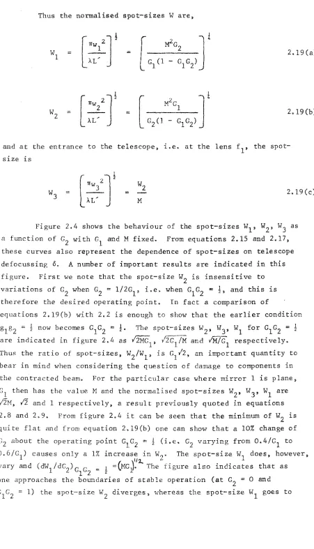
(36) 29. loss of 0.01, the TEM^ (1 - Lgg/l ". loss is 0.12, thus giving a value for. of ~60 for q = 35.. Despite this large selectivity it must be borne in mind that the mode-selection is a sensitive function of hence of aperture size.. and. and. It is therefore advisable, in selecting. the aperture size, to have available a range of closely spaced aperture sizes so that one can find in practice w h i c h gives the most satisfactory performance.. Using the parameters already quoted for. our resonator and the aperture diameter 2a = 6.25mm, the above expression for Fresnel number yields the value 0.74.. With this. Fresnel number, Li's calculations give round trip losses for our resonator of. = 0.008,. = 0.10, thus giving a generous degree. of mode-selection over the 35 or so round trips w h e n Q-switched. The very small diffraction loss for the TEM. mode suggests that little. or no diffraction ring structure would be visible in the output beam since the mode is only very slightly truncated.. This is indeed the. case and figure 2.8 shows a sequence of burn patterns on photographic film.. These were taken at 4m from the output resonant reflector.. Figure 2.9 shows the TEM. mode intensity profile as observed on a. diode array, confirming the smooth, structureless profile indicated by the b u m. patterns.. Spot-sizes measured using the diode array. agree within experimental accuracy with TEMg^ spot-sizes predicted by our analysis..
(37) 30. Figure_2.8;. Sequence of burns on photographic paper.. These were. taken at 4m from the resonant reflector, at an output energy of 'V'lOOmJ, and a repetition rate of 8H2. t *:. Figure 2.9:. TvL I ;. Beam profile as monitored by a diode array.
(38) 31. 2.4. Thermal Lensing of Che Pockels Cell Q-Switch It was noted in section 2.2.3 that the Pockels cell can. contribute an additional negative lens to the cavity as a result of absorption of the laser radiation. optimum telescope defocussing,. This effect modifies the via equation 2.25.. This lensing effect was noticed early in the experimental programme on the telescopic resonator as a result of tha cavity alignment procedure being used at that time.. Satisfactory results. as regards beam divergence and profile had been obtained with the laser operating fixed-Q with an output energy of 350%^ without a Pockels cell in the cavity.. The Pockels cell was then introduced. into the resonator and the laser operated without any voltage applied to the cell. bum. A degraded beam profile (assessed by visual inspection of. patterns taken on blackened photographic paper) was observed.. This led us to believe that the Pockels cell was acting like a lens, with the result that the telescope spacing was no longer optimised. However, use of a Mach-Zehnder interferometer indicated that the cell crystal faces were polished plane parallel to better than X / 8 at 1.06wm, so we concluded that the lensing effect w a s induced as a result of absorption of the laser radiation.. The resonator. configuration used to confirm this is illustrated in figure 2.10. The cavity is formed by a 5m radius 100% reflectivity mirror, and a plane 30% reflectivity mirror which served as the output coupler. A 7.5mm diameter aperture was used to restrict oscillation to the TEMgQ mode when the resonator was in optimum adjustment. energy was 42J and the repetition rate was 17.5Hz.. The pump. The laser output. energy was measured as a function of telescope lens spacing for the two cases:. (1). with the Pockels cell present, and. (2). with the Pockels cell removed from the cavity.. For each telescope setting the 5m radius mirror w a s adjusted to re-optimise the cavity for maximum output.. For convenience, the output energy was. measured using a J.K. Lasers energy monitor.. This instrument is only in.
(39) 1'35ni 0'55m. E I. (a). (b). (c). (d). (e). (f). (g). (Q) Mirror. 5m radius, 100% reflectivity. le) Aperture. 75mm dia.. (b) Telescope. Magnification = 4. (f) Laser rod.. (c) Position of Pockels cell.. (g) Mirror. Plane, 30%. (d) Dielectric polariser. Figure 2\10:. reflectivity.. The fixed-Q telescopic resonator used to measure the shift in optimum telescope lens spacing as a result of thermal lensing in the Pockels cell. lengths of the telescope lenses were +20cm and -5cm. The focal w N.
(40) 33. rough calibration, and consequent]y the results, illustrated in figure 2.11, are normalised, in each case, to the maximum output energy.. Figure 2.12. shows the corresponding burn patterns taken ~30cm from the output coupler, and in conjunction with figure 2.11 clearly shows a shift of ^+2mm in the optimum telescope lens spacing. One can easily show from equation 2.25 that the change in optimum telescope lens spacing, ^6^. caused by. addition of a. Pockels cell of focal length f , is given by. A6. opt. =. - — _ ^. 2.31. For our set-up w e have A6 = 2mm, f_ = 20cm, giving f = -20m. ^ opt 2 * ° p An analysis of the thermal lensing exhibited by absorbing elements in a laser beam has been performed by Gordon et al. (1965). They derive the following expression for focal length, f, of an absorbing sample when placed in a Gaussian laser beam of average power P, and spot-size. w, using the simplifying assumption that the change. in refractive index of the sample is parabolic with radial distance from the beam axis.. 2.32 apt dT. In equation 2.32 k is the thermal conductivity, n is the refractive index, a is the absorption coefficient and & is the length of the sample.. This expression is valid provided two conditions are met:. (i) that only changes in refractive index contribute to the focussing effect, i.e. that changes in the physical dimensions of the sample have no effect; (ii) that the time between laser pulses is much less than a characteristic thermal relaxation time constant given by. t ^. where D = k/PC density and C. =. — 4D. 2.33. is the thermal diffusivity of the sample, P is the the specific heat.. Using w = 2.5mm and values for the.
(41) X. -. Cavity without Pockels cell Ccivity v/ith. 1/. Pockels cell. — I r n m r""— Telescope lens spacing (Increasing—*-) Figure 2.11:. Normalised laser output energy as a function of telescope lens spacing, measured before and after addition to the cavity of the Pockels cell. w.
(42) Figure 2.12:. A sequence of b u m. patterns illustrating the shift in optimum telescope spacing upon. insertion of the Pockels cell.. The upper sequence was obtained without the Pockels cell. in the cavity, the lower sequence with.. The braces indicate the region of telescope. CO. Ul adjustment over which acceptable profiles were obtained in each case.
(43) 36. other constants appropriate to KD*P for convenience)5 we find t condition. (these are listed in table 2.1. = 1.7s.. (ii) is certainly met.. Since we are working at ^ISHz,. Furthermore, the crystal is immersed. in a refractive index matching fluid, therefore curvature of the crystal faces caused by thermal expansion will not contribute to the focussing effect, and so condition (i) is also met. To use equation 2.32 to calculate the induced focal length, we need Co know the value of absorption coefficient for our crystal.. The. absorption coefficient of KD*P depends on the degree of deuteration, varying linearly from a = OUlZcm"! for undeuterated KDP to a = 0 for 100% deuterated KD*P. (R. Wood, Private Communication).. Unfortunately,. the exact deuteration for our crystal is not k n o w n , but for the purpose of calculation we assume a typical figure of 957,, giving & = 6 x 10 ^ cm ^ . Inserting values from table 2.1 into equation 2.32 gives f = -22m, where we have used P = 5.2W. (corresponding to SOOmJ laser. output at 17.4HZ) and A = 1,5cm for our Pockels cell crystal.. This. agrees well with the experimental measurement of f = - 2 0 m , but this must be regarded as fortuitous since we have, in calculating the power incident on the Pockels cell, assumed in effect that the Pockels cell is mounted outside the laser resonator.. In practice, the relationship between. output power and the power which circulates each w a y through the Pockels cell is not straightforward, and may be significantly different from the simple estimate of 5.2W we have used above. As a result of this observation of Pockels cell lensing, we now take the additional precaution in the alignment procedure of plotting output energy against telescope lens spacing.. A f t e r first. setting the telescope lens spacing for perfect adjustment for visible light using an autocollimater, an additional calculated adjustment is made to compensate for dispersion in the lenses.. Using equation 2.25,. the required value of 6^ ^ is calculated and also introduced to the lens spacing.. The resulting spacing is usually sufficiently accurate. for laser action to occur once the resonator mirrors are aligned.. A. plot of output energy vs. spacing accompanied by a sequence of burn patterns then allows the optimum setting to be found.. Once set in this. way, no further adjustment of the telescope should be necessary, and any change in operating conditions of the laser such as repetition rate or pumping energy can be compensated for by adjusting the telescope lens spacing according to equation 2.25..
(44) 37. Table 2.1:. Some optical and thermal properties of KD*P. REFERENCE. VALUE. Thermal conductivity, k. (a). 1.88 X lO-^cm'^K"^. Heat capacity, C. (b). 0.87jg"'^K''^. Density, P. (b). 2.34 gcm"^. dn/dT. (c). -5.1 X 10"%"^. (d). 1.47. QUANTITY. Ordinary refractive index, n ^. (a). |. Y.S. Touloukian et al., 1970.. Value measured at T " 300 K,. parallel to optic axis. (b). C.J. West and C. Hull, 1933.. (c). M. Yamazaki and T. Ogawa, 1966.. (d). W. Koechner, 1976.. Value calculated at T = 300°K..
(45) 38. 2.5. Mode Selecting Apertures: A Practical Point Concerning Their Design The mode selecting apertures we have used in our work on laser. resonators are made by drilling a hole of the required diameter in a flat disc of brass or steel, and then countersinking one side, as shown in figure 2.13.. During our work we found that the laser would only. function reliably with TEM^^ mode output when the countersunk side of the aperture faced the laser rod (see figure 2.14(b)).. This behaviour. has been observed both with the telescopic resonator using a 6.25mm diameter aperture and also with resonators. incorporating. conventional small volume TEM^Q mode. 2mm diameter apertures.. We illustrate this in figure 2.15, where we show Q-switched burn patterns at the 80mJ output level.. These were obtained using the. telescopic resonator referred to in section 2.2.3 and discussed more fully in Chapter Three.. The aperture is situated between the laser. rod and the 100% reflectivity mirror, and the laser output is taken from the contracted beam end of the laser.. One can clearly see a. tendency for the laser to break into TEM^^ mode oscillation with the aperture arranged as in figure 2.14(a). In the telescopic resonator it was possible to induce this behaviour only by adjusting the aperture to be off centre from the beam axis.. In the conventional resonator, however, this behaviour. was always observed when the countersunk side of the aperture faced fi^m the laser rod, regardless of aperture centring, and oscillation was occasionally observed on imodes of higher order, up to TEM^ . It would appear that this behaviour is due to feedback from the plane face of the aperture and mirror. (see figure 2.14(a)).. figure 2.14(b), any light incident from the left on the aperture is reflected out of the cavity by the chamfered lip on the aperture, thereby suppressing oscillation. This is clearly a point of some practical importance in the design and setting—up of a laser oscillator since it may not be immediately obvious that poor laser performance can result from incorrect aperture design or orientation.. In.
(46) 39. 1 6mm 2a mm Figure 2.13:. figure 2.14:. Cross-section of a mode-selecting aperture. The two possible orientations of. the aperture. relative to the laser rod and resonator mirrors, M. and Mg.
(47) 40. ah. m m m m m. m m. E N 5 r _. Figure 2.15:. A sequence of burn patterns illustrating the effect of having the aperture oriented as shown in figure 2.14(a).
(48) 41. 2.6. Pockels Cell Alignment The correct alignment of the Pockels cell crystal relative to. the laser beam is with the crystallographic x or y axis parallel to the polarisation vector and the z, or optic, axis parallel to the propagation direction.. When aligned in this way, the crystal behaves. isotropically with zero applied voltage, and therefore does not alter the polarisation of the laser beam.. However, if the z axis is misaligned,. the resulting optical anisotropy can lead to a cavity loss via the intracavity polariser.. Since the crystal is uniaxial under zero field. conditions, orientation of the x and y axes is unimportant as regards cavity loss.. (A field-dependent phase shift effect caused by x, y. axis misalignment is di scussed in section 4.3.3.). 11 is useful,. therefore, to derive an expression for cavity loss as a function of angular misalignment of z axis from propagation direction. The system of coordinates is shown in figure 2.16.. XZ is the. plane of polarisation of the laser beam and Z is the propagation direction.. The optic axis makes an angle. direction, and an angle. X. 8. with the propagation. with the plane of polarisation.. By varying. X with 6 fixed, one finds that the greatest power loss from the polariser in figure 2.17 occurs for values of X obeying X = (90n + 45)°; n = 0, 1, 2, 3.. For our worst-case calculation of alignment tolerance. we will take X = 45°.. One can write the phase shift between the. ordinary and extraordinary components of the b e a m after passing through a length. &. of crystal. 2.34. (ngCG) - n^). wh^re n (8) and n are the extraordinary and ordinary refractive e o indices, n (8) is related to 8 by the following expression. sin 0 ^ cos n. 2.35. n. which after some manipulation can be rewritten -I 1 +. (n^ - n^) o e. . 2a sinTo. 2.36.
(49) 42. Optic axis. Eigure_2^16:. System of coordinates used in the evaluation of cavity loss as a result of Pockels cell misalignment. L Crystal. Figure 2.17:. The Pockels cell crystal inside the laser cavity.
(50) 43. n. In general, n'. will be much smaller than unity, and also, since. we are considering small misalignments, sin'. «. 1.. We can. therefore write. n^(e) -. I ("e. 2.37. "o)("e + % ). 2n. Furthermore, since n^ = n , we can simplify equation 2.37 further. n (8) - n e o. (n. e. 2.38. - n ) o. The Pockels cell inside the laser cavity is shown in figure 2.17.. The. effective crystal length is 2& since light passes twice through the cell on each round trip.. One can easily show that the transmission of. this optical system is given by. 2.39. (1 + cosO). K From equations 2.39, 2.38 and 2.34 we can write the transmission T as a function of 8. 1 + cos. I. 4%%. 2.40. This is illustrated in figure 2.18 using the following parameters: & = 1.064wm, and for our crystal & = 1.5cm, n - n = 0.04. ' e o. If we take. as our criterion for low loss operation that the transmission must be greater than, say, 0.95, we therefore require 8 < # m r a d .. N o w 8 is. measured internally, so the external alignment angle is greater by a factor of n , i.e. 8. < l2mrad.. The Pockels cell alignment procedure we h a v e used in the course of our work involves centering the 'Maltese cross' pattern (see e.g. Koechner, 1976) on the resonator axis.. This is done by illuminating. the crystal with a He-Ne laser beam which has first been carefully aligned parallel. to the resonator optical axis.. The beam is diffused. by passing it through a lens tissue, resulting in a bright central spot surrounded by scattered light.. When the crystal is placed between. crossed polarisers, a pattern of a dark cross surrounded by a series of.
(51) 0 (mrad) Transmission, T, of the Pockels cell/polariser combination shown in figure 2.17 as a function of crystal tilt, 0.
(52) 45. circles appears (see e.g. Bomn (Hid Wolf, 1975).. The line connecting. the centre of the cross to the lens tissue is parallel to the z axis.^ The Pockels cell is now brought into alignment by tilting it so that the centre of the cross coincides with the bright unscattered component of the He-Ne beam.. When this is performed carefully we estimate that. it is possible to align the Pockels cell optic axis to the resonator axis to better than 2mrad (measured externally to the crystal). this is well within the required criterion 8. Since. < 12mrad, we conclude ext. that Pockels cell losses as a result of crystal misalignment should be negligible in practice.. 2,7. Conclusion We have ended this chapter by introducing some additional. discussion of three practical points mentioned only briefly in earlier sections.. We show that under conditions of high average power laser. operation that absorption of the radiation by the Pockels cell can induce a thermal lens of sufficiently short focal length to require a correction to the lens spacing of the telescope, and provide an approximate expression which can be used to estimate the significance of this effect.. Furthermore, our practical investigations have led us. to adopt a particular design and orientation of m o d e selecting aperture: if incorrectly designed, significant distortion of the transverse mode occurs.. Finally, an estimate of the angular alignment tolerance on the. Pockels cell is made, and the alignment procedure w e have adopted, the "Maltese cross" method, is described. Thus, in conclusion we have shown that a telescopic resonator can provide a reliable means of generating a large volume TEM. mode in a. NdzYAG laser, permitting Q-switched operation at the lOOmJ level.. An. analytical description of this type of resonator has been developed which reduces to a few simple design equations.. We have found that these. equations describe the experimentally observed behaviour with a degree of completeness and accuracy beyond what was expected. a. This indicates that. thorough design calculation could be made, e.g. to maximise. output energy while keeping clear of damage problems, and the results of. This is only strictly true if the crystal faces are polished perpendicular to the optic axis..
(53) 46. such a calculation could be trusted with confidence.. It is expected. that a similar exercise could be extended to other optically pumped solid state lasers, notably Nd doped glass and ruby..
(54) 47. CHAPTER THREE. EXPERIMENTAL WORK ON THE TELESCOPIC RESONATOR. 3.1. Introduction In this chapter we consider the experimental development of. the telescopic resonator. Of central importance to our investigation of the telescopic resonator is the measurement of angular divergence and intensity profile of the output beam, since these give a quantitative and objective measure of the transverse mode structure.. We therefore begin. this chapter with a discussion of techniques which m a y be used to perform these measurements, and describe the technique which w e have developed to allow their accurate and quick determination. A previous investigation of the telescopic resonator by Herbst et al. (1977) gave poor results as regards transverse beam quality and output energy.. Our own initial problems with the resonator. have led us to adopt a careful alignment procedure, of which we give a detailed account in section 3,3.. We conclude the chapter with the key. results of the experimental programme on the resonator.. 3.2. Beam Spot-Size and Divergence Measurements: Method To provide a framework for discussion of experimental techniques,. we begin this section by making some general points concerning the diffraction behaviour of Gaussian beams. Suppose a laser oscillates only on the T E M with a spot-size at the beam waist, w .. transverse mode,. For such a beam, the angular. divergence is given by. 8. =. ^. 3.1. ""o. and the spot-size at a distance z from the waist I . 2. w(z). =. WQ \ 1 +. A. 2. 3.2. •"OJ (see, e.g. Kogelnik and Li, 1966).. Consider the situation where the.
(55) 48. beam has propagated to the far field, which we define by the condition 2 Xz. ». 2 ""OJ. 1. 3.3. In this case, one can write, using equations 3.2 and 3.1. w(z). =. =. 8. 3.4. %. In principle, then, one would measure w distance z satisfying equation 3.3.. at the waist, and w(z) at a. The calculated value of 8 from. equation 3.1 is then compared to w(z)/z.. If they are equal, we say. that the beam is 'diffraction limited'. There are, however, three major problems which arise when we attempt a practical measurement of these quantities.. (a). To measure the spot-size, one requires to measure the intensity profile of the beam.. How can this be performed reliably,. quickly and accurately? (b). The measurement of w_ in the scheme outlined above relies on 0 the laser forming a waist outside the cavity.. For general. applicability, however, one needs to devise a scheme which can handle the situation where the waist is formed inside the cavity. (c). One may have to allow the beam to propagate inconveniently far to reach the far field.. This can be seen by considering a = 2mm, X. typical laser output characterised by. -. lym, for. which the condition for far field diffraction is z ». 13m.. The intensity distribution in the laser beam can be monitored in three ways.. (i) The beam can be photographed.. After development,. the resulting image is analysed using a microdensitometer.. When using. this technique great care must be exercised to ensure operation on the linear portion of the film characteristic, and subsequent development and analysis of the image is time consuming.. (ii) A detector mounted. behind a pinhole can be moved mechanically across the beam on a calibrated, accurate translation stage.. This m e t h o d , however, requires. a lot of laser operation time, and gives no information on the intensity.
(56) 49. profile of a single laser pulse.. (iii). The beam. using a scanning photodiode array (S.P.A.).. be monitored. In this technique, the. intensity distribution of the incident beam is 'stored' on a linear array of silicon photodiodes, which are then sequentially sampled and displayed on an oscilloscope.. In this way it is possible to monitor. the profile of an individual laser pulse.. Furthermore, the control. electronics is set to clearly indicate when the diodes are operating outside the region of linear response.. For these reasons we have chosen. to use an S.P.A. for our measurements of beam profile, and therefore restrict out later discussions to the use of this instrument. The problem of propagation to the far field may be overcome by focussing the beam, as illustrated in figure 3.1.. W e note that the. beam waist is not, in general, formed in the focal plane of the lens, but at a distance which depends on the spot-size w and wave front curvature R of the beam which is incident on the lens.. This. can be seen by considering the lens as consisting of two parts, the first of which corrects the wavefront curvature and presents plane wavefronts to the second, of focal length f^ = (l/f - 1/R) ^.. One can. then show that the beam waist occurs at a distance z. = f /(I + (Xf'/ww^)) from the lens. As a result of the high degree of collimation of a laser beam,. the diameter of the beam waist formed after passing through a lens is very small for typical, practical values of lens focal length. illustrate this we assume that a beam, spot-size w back focal plane of a lens of focal length f.. To. , is incident on the. The beam is focussed to. a waist w ^ ^ in the fi front focal plane of the lens.. It is easy to show. that Wg^ is given by. • ". •. %. Taking typical values for w^, & and f (appropriate to our experimental arrangement) of 2mm, IWm and Im respectively, we find from equation 3.5 that w. = 160wm.. Our S.P.A. has a diode spacing of lOOWm, and if this was. placed at the beam focus to monitor the profile, the spatial resolution would be clearly inadequate.. We therefore image the waist. with a second lens, arranged to give a magnification M > 1.. The general. experimental arrangement we have used is shown in figure 3.2, where for.
(57) Figure 3,1;. Use of a lens, focal length f, to form a beam waist at a distance from the lens g.
(58) Experimental arrangement used to measure the waist spot-size,. , and. profile formed by a lens of focal length f. Ln.
(59) 52. clarity various attenuators have been omitted.. The. incident from the left on a lens of focal length f waist with spot-size w^^, at a distance z in general z. f f^.. laser beam is and brought to a. from the lens.. Note that. Having located the waist formed by this first. lens a second lens of focal length f^ is used to image the waist onto the S.P.A., giving an image spot-size w^ = Mw^^, w h e r e M = v/u is the geometrical magnification.. This can be measured b y examining the. signal from the photodiode array, and w. deduced from w ^ = w\/M.. If. the incident beam were a pure T E M ^ mode then the spot-size w^ at lens 1 would be given by equation 3.2 with z. Zg and w. w.. Of. This. calculated value is compared with the measured value of replacing lens 1 with the S.P.A.. obtained by. If equal, then the beam is diffraction. limited. In practice, there is always an. error. location of the waist formed by lens 1, and the S.P.A.. In this case, w^ # ^ O f. 6^. associated with the. an error 6^ in the placing of. the object plane of the. imaging system no longer contains the waist.. To calculate the. magnitude of this effect, we find the beam magnification, defined by M. = ^i^^of'. the arrangement illustrated in figure 3.3.. By using. the ABCD law for Gaussian beams (Kogelnik, 1965), one can show that M ' is given by. 2 M. -. X. M Mfg. Mfg l"'. ""Of 3.6. Clearly, when the system is in perfect alignment, i.e. when 5 then M. = M - v/u as required.. 6^/Mfg << 1, 2' 2 expression.. = 6^ = 0,. For the practically important case. << 6 , we can write a more compact, approximate. M. M. 1 +. 3.7 TTw Of. As an example, consider our earlier illustration, where a waist of 160Wm diameter was formed by a Im focal length lens.. In our. experiments we have found it convenient to use a m a g n i f i c a t i o n M - 7, accomplished by using a 15cm focal length lens w i t h u " 17.1cm, v - 120cm. To locate the small beam waist we have used either an infra-red phosphor.
(60) V + S'. Errors 6^ and Gg in the object and image distances u and V. Ln w.
(61) 54. card or exposed photographic paper, with an estimated accuracy of <5^ = ±2cm.. Inserting M = 7, A = Ipm, w. gives M ' = 7.2.. = 160pm into equation 3.7. This would give rise to an error in deducing w^^ of. 0.2/7 5 3%, thus illustrating the high degree of accuracy that one might expect in beam divergence measurements performed by this method.. 3. 3. Cavity Alignment Procedure. 3.3.1. Telescope alignment When setting up a telescopic resonator, one of the most. important aspects of alignment is finding the correct telescope spacing. In the course of our work we have found that this can be easily and conveniently achieved in two stages.. (i). The spacing of the lenses is first adjusted so that the. telescope is exactly collimated.. This is achieved by viewing a plane. mirror through the telescope using an autocollimator. is then adjusted wires.. The lens spacing. to form a sharp image of the autocollimator cross. A calculated correction is now made for dispersion, using the. dispersion formula for BK7 glass (the material used for our telescope lenses).. This is given in the Schott glass catalogue as. n% A. =. A. =. 2.2718929. A. =. -1.0108077 X 10"2. A. =. 1.0592509 x lo"*. A. =. 2.0816965 x lO"^. A^. =. -7.6472538 x 10"^. Ar 5. =. 4.9240991 x 10"?. 0. + A^X-2 + 2. 1. + A/X'S + AcX-^ 4 5. 3. where. where & is in microns.. We assume that by using the autocollimator,. the telescope is correctly adjusted for & ~ 500nm, and so the required correction is n r - n_ ^1.06 - °.5. -. d.5 :. To this is added the design value of 6 2.25.. 3 X 10. '. "1.06. 2. 1 ^ calculated using equation.
Figure
Related documents