The unsteady forces on slender delta wing hydrofoils oscillating in heave

THE UNSTEADY FORCES ON SLENDER DELTA WING HYDROFOILS OSCILLATING IN HEAVE

Thesis by Raymond Kay DeLong

In Partial Fulfillment of the Requirements for the Degree of

Doctor of Philosophy

California Institute of Technology Pasadena, California

1968

(Submitted 24 May 1968)

*

•

I would first like to thank Professor Allan Acosta who served as my advisor during my graduate study and without whose assistance this thesis would not be possible.

I would also like to express my gratitude to the Institute and to Douglas Aircraft Co., Inc. (now part of McDonnell Douglas

Corporation) for the financial aid received during my stay here. In the course of my investigations I wrote letters to many people inquiring about their work. To those who were kind enough to take the time to answer I say, "Thank you".

The undertaking of any experimental investigation of the scope herein discussed must always require the participation of others. In particular I would like to thank Mr. R. Lyon of the Institute's Central Engineering Services and Messrs. C. Eastvedt, H. Hamaguchi,

J. Kingan and G. Lundgren of the Hydrodynamics Laboratory. The assistance of Miss Cecilia Lin, Mr. H. Petrie and

Mr. M. Wilson in the preparation and proofreading of this manuscript is gratefully acknowledged.

And finally, to Mrs. Phyllis Henderson, former secretary for the Hydrodynamics Laboratory and still my good friend, who so

THE UNSTEADY FORCES ON SLENDER DELTA WING HYDROFOILS OSCILLATING IN HEAVE

by

Raymond Kay DeLong

ABSTRACT

The investigations described herein are both experimental and theoretical. An experimental technique is described by which the models tested could be oscillated sinusoidally in heave. The

apparatus used to gather the unsteady lift, drag and pitching moment data is also described.

The models tested were two flat delta wings with apex angles of 15 ° and 30 0 and they had sharp leading edges to insure flow

separation. The models were fabricated from 0.25 inch aluminum plate and were approximately one foot in length.

Three distinct types of flow were investigated: 1) fully wetted, 2) ventilated and 3) planing. The experimental data are compared with the existing theories for steady motions in the case of fully wetted delta wings. Ventilation measurements, made only for the 30 0 model at 20 ° angle of attack, of lift and drag are presented.

A correction of the theory proposed by M. P. Tulin for high speed planing of slender bodies is presented and it is extended to unsteady motions. This is compared to the experimental measure-ments made at 60 and 12 0 angle of attack for the two models previously

This is the first extensive measurement of unsteady drag for any shape wing, the first measurement of unsteady planing forces, the first quantitative documentation of unstable oscillations near a free surface, and the first measurements of the unsteady forces on ventilated delta wings. The results of these investigations, both

theoretical and experimental, are discussed and further investigations suggested.

•

TABLE OF CONTENTS

Page Acknowledgments

Abstract

Table of Contents I. INTRODUCTION

ii iii v 1

A. Preliminary Remarks ₁

B. Previous Investigations ₄

C. Present Investigations ₁₀

II. EXPERIMENTAL APPARATUS ₁₃

A. Free Surface Water Tunnel ₁₃

• B. Hydraulic Pump and Oscillator ₁₄

C. Servo Controller

14

D. Models and Attachment Fixtures ₁₅

E. Instrumentation ₁₅

1. Lift and Pitching Moment Balance ₁₅

2. Drag Balance ₁₆

3. _{Voltage Supplies and Amplifiers}

18

4. Return Signal .Analyzer ₁

9

6. Digital Voltmeter ₂₀

7. _{Position and Velocity Transducers}

20

F. Support and Ventilation Struts ₂₀

G. Ventilation Measuring Apparatus ₂₁

• 1. _{Air Supply Measurement}

•

Page

2. Cavity Length Measurement ₂₁

3.

III.

A. Calibrations

₂₂

1. Position Transducer

₂₂

2. Velocity Transducer

₂₂

3. Lift and Pitching Moment Balance

₂₂

4. Drag Balance

₂₃

5. Return Signal Analyzer

₂₄

6. Air Supply Apparatus

₂₄

B. Parameters Investigated

₂₅

•

₂₇

D. Data R eduction

₂₉

1. Force Coefficients ₃₀

2. Ventilation Parameters

₃₅

IV. A THEORY OF UNSTEADY PLANING OF SLENDER

BODIES AT SMALL ANGLES OF ATTACK ₃₆

A. Preliminary Remarks ₃₆

B. _{The Coordinate System and Bernoulli Equation 36} C. Laplace's Equation and the Boundary Conditions

₃₉

D. Approximations

₄₀

E. _{The Solution of the Boundary Value Problem}

₄₄

F. The Calculation of Forces ₄₉

G. Specific Cases

₅₈

• _{H. Conclusion}

e

V. DISCUSSION OF THE EXPERIMENTAL DATA

Page

AND THEORETICAL CALCULATIONS ₆₃

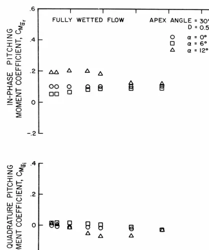
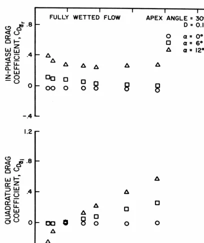
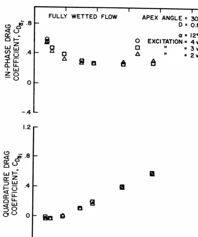
A. Fully Wetted Flow ₆₃

B. Ventilated Flow ₆₈

C. Planing Flow ₇₀

D. Part-Cycle-Planing ₇₃

VI. SUMMARY AND CONCLUDING REMARKS 75

References ₇₇

Figures ₈₀

Appendix - List of Symbols and Notation 135

•

A. Preliminary Remarks

A hydrofoil boat is one which derives its lift force primarily from "wings" mounted to and away from the boat's hull. _{The lift is} generated by the acceleration of the fluid surrounding the foil. _This situation is very similar to an airplane flying through the atmosphere and much terminology and technique applied to hydrofoil boats has its roots in aeronautics.

•

Conventional boats, commonly called displacement craft, are buoyed up by the static pressure of the surrounding fluid. _{The boat} displaces an amount of water equal to the boat's weight, hence the name displacement craft. _{All conventional hydrofoil boats operate in} two modes. _{At low speeds (e.g., when docking) they operate as dis-} placement craft and may or may not have their foils retracted. _At higher speeds (e, g., design cruise) the hull is lifted clear of the water and the entire force is generated by the hydrofoil system. _In this mode the craft is said to be "flying".

The idea of using hydrofoils on boats is not new. _{It was first} considered prior to the turn of the century. _{Even in 1919 Alexander} Graham Bell, who is considerably more famous for another achieve- ment, had built and operated a hydrofoil boat capable of 60 knots.

•

•

-2-

over displacement craft. Displacement craft operate on the surface of the water and as a result are greatly affected by the surface waves generated by wind, other boats, etc. A hydrofoil boat can operate with its hull above the wave crests and its foils submerged far enough so that the waves affect the lift to a negligible extent. The result is that a hydrofoil boat has better seakeeping capability at high speeds than does a displacement craft.

This increased immunity to surface conditions is beneficial in both military and commercial applications. Currently the most likely military application is as a submarine chaser where the hydrofoil

craft's ability to travel at high speeds in relatively rougher seas makes it a better choice. In commercial applications the dimunition of the wave influence gives a smoother ride. The decreased loading allows less fortress-like designs; indeed, since the craft operates somewhat like an airplane it must necessarily be built as light as possible,

otherwise the operating range would suffer from the extra weight. Various hydrofoil configurations are popularly used. These are described in the voluminous monograph of Abramson, et al (1).

There are several basic types of foils used in various combinations. These are planing, deeply submerged and surface piercing. The total lift generated by the foils is not affected by their _{placement since the}

lift generated must in any event equal the weight of the craft.

The types of foils used and their arrangement will govern the stability of the craft, however. A planing foil has stability as long as

•

•

area but is obviously severely affected by the surface waves. A submerged foil will experience a decrease in lift as it nears the free surface but the effect is slight unless the foil is less than a fraction of a chord from the surface. Ladder foils and surface-piercing V-foils are much better in that they can be designed to give whatever quasi-steady stability is desired.

The type of stability discussed in the previous paragraph con-cerned the craft's natural tendency to return to the trim condition when perturbed. If the craft is suspended at three non-collinear points and the foils at each point have heave stability, the craft will also have pitch and roll stability. The pitch and roll "stiffness" depends on the separation of the points. The greater the horizontal • distance between the foils the stiffer the suspension.

So far we have only been concerned with the lift force. For a boat which is to go other than in straight lines some means must also be included to generate side force for turning. In an airplane this side force is produced by banking the wing. This can also be done on a hydrofoil boat, but due to the interaction of the free surface it

usually is not. What is generally done is to have the support strut generate the side force for inverted T and inverted ir foils and for V-foils differential lift in the two halves may be used to generate

side force. The latter system is used on the tail of a Beechcraft Bonanza airplane.

The infinite variety of ways in which the problem of building a hydrofoil boat can be attacked is part of what makes the problem

e

-4-

of the designer's problems is clearly beyond the scope of these introductory remarks and the entire thesis.

We will now confine ourselves to one facet of the design of hydrofoil boats, and that is its motion about its steady flight. If the boat is caused for any reason to oscillate about its mean path, the unsteady motion of the foils will give rise to unsteady forces caused by the acceleration of their fluid environment. The interaction of these elements (1. e,, fluid and foil-boat system) is commonly called hydroelasticity.

Before an analysis can be made of the motion of the craft, a quantitative specification must be made of the forces experienced by the foils for various motions. It is the endeavor of this thesis to • add to the still rather sparse quantity of information regarding

unsteady hydrodynamics.

This investigation has been primarily concerned with delta planforrn foils and as such the work of previous authors will be for the most part also concerned with delta wings. References to other work will easily be found in references (1), (2) and (3).

B. Previous Investigations

The interest in triangular lifting surfaces hardly needs

justification. They are common in aeronautics and from the studies of persons whose primary interest was motivated by aeronautical consideration we will consider previous "fully wetted" flow results. As was mentioned by Smith (4) the effect of Reynolds number on the

•

•

-5-

Although viscosity is the physical property which determines the smooth outflow or lateral Kutta-Joukowski condition, the absolute value of the viscosity is not too important as long as the Reynolds number is moderately high.

Prior to the interest in flows about delta wings with leading edge separation R. T. Jones (5) presented a method for calculating the force on a slender body at small angle of attack. Jones' analysis, conducted in the cross-flow plane, is applicable to slender delta wings. The cross-flow plane solution used was for a flat lamina perpendicular to the flow. The infinite velocities at the lateral edges in this model clearly do not exist in the actual case. Jones' analysis is, however, satisfactory for slender delta wings at small angles of attack and his

1110

to be linear with angle of attack.

Subsequent experimental investigations, particularly by Roy (6), caused interest in finding a model which represented the observed flow especially the smooth outflow condition at the leading edges.

Legendre (7) proposed the addition of two vortices above and inboard of the two leading edges. The strength and position of the vortices would be determined by the smooth outflow condition at the leading edges with the condition that the vortices have no net force on them. The two vortices were implicitly assumed to be joined by a cut so that the lift on the foil or foil-vortex system would be uniquely determined.

- 6-

•

vortex. His force condition was still on the vortex which meant that the lift on the foil depended on whether the forces or the cuts were included or not.

Brown and Michael

₍₉₎

Edwards (1 _{0), which placed the zero force condition at each vortex on} the cut as well. That is, the net force on the vortex and cut taken together should be zero. The ambiguity in the lift calculation was then removed.

The Brown and Michael model has served as a basis for a number of other investigations. It has the advantage of basic

simplicity and it reasonably represents the flow picture. It does not, • however, predict the forces very well, being somewhat too high.

The stability derivatives are likewise poorly predicted.

Trying to develop a model which was even closer to the

physical flow and one which would better predict the forces, Mangler and Smith (11) proposed a model with the flow separated from the leading edge being represented by a spiral vortex sheet. Somewhat better agreement with experimental data was obtained than with the Brown and Michael model. It has the disadvantage that the added complexity requires that the problem be solved on a _{digital computer.} Smith (4) has recently published some further calculations using this model. These are used in the discussion of the experimental results in Section V.

•

-7-

Gersten's method is basically one of lifting surface theory. It has the advantage that it predicts the forces fairly well but it has the aesthetic disadvantage that the trailing vortex field of his lifting surface theory does not physically resemble the actual flow.

These are the major efforts to predict the steady forces on fully wetted delta wings. There have been other studies of the vortex structure and some flow visualization studies, particularly Marsden, et al (13), but these are the models from which most current work extends. The studies in this area are currently active as will be

noted by Kiichemann.'s (14) report on the 1964 I. U. T.A.M. symposium held at Ann Arbor, Michigan. Several of the papers, notably (15),

(16) and (17), presented at this symposium have since been published in volume seven of Progress in Aeronautical Science. Also the work of Garner and Lehrian (18) is notable but is really derived from Gersten' s.

In the area of unsteady loads on non-stationary delta wings Jones' idea was discussed by Miles (19) and Garrick (20) for the linear problem. The unsteady problem with leading edge separation has been treated by Randall (21) who used the Brown and Michael model to calculate the force on a slender delta wing performing

•

-8-

Randall shows encouraging agreement. Due to the computational difficulties no extension of the more realistic Mangler-Smith model has been made to unsteady flows but it would undoubtedly give

superior force predictions.

Another investigation of the forces on delta wings oscillating in heave was presented by Lawrence and Gerber (24). They used slender wing theory to calculate the effect of reduced frequency on the unsteady forces on some rectangular and delta wings. The theory is limited to vanishingly small angles of attack, not a very practical case, but gives surprisingly good correlation within the bounds of the theory. This is discussed in Section V.

The other two types of flow investigated herein are unique to • hydrodynamics, therefore no aeronautically inspired results will be available. The second flow type (1. e., ventilated or cavitating) has received but slight treatment for delta wings. Tulin (25) has

presented a theory for slender partially cavitating delta wings. This was subsequently corrected by Kaplan, et al (26). This model,

though interesting, is not applicable to the current study since only a fully ventilated foil was tested.

cavity..-foil system in the cross-flow. The computational details of the theory are fairly tedious. Extension of this approach to unsteady flows would seem to be very difficult. Experimental investigations of cavitating delta wings were performed by Reichardt and Sattler (28). They indicate poor correlation with the Curnberbatch-Wu theory but due to the small size of the models the results of the experiment are not unquestioned. An experimental investigation of the forces on

steady ventilated delta wings by Kiceniuk (29) indicates fairly good agreement. The problem seems to be open for more detailed res earch.

The third type of flow investigated herein is planing of slender delta wing hydrofoils oscillating in heave. _{Planing of delta wings has}

0

interested in V-bottom hulls with some work being done on rectangular skis for operation on water-based aircraft. _{Some delta configuration} foils were investigated for use on hydro-ski aircraft but they were mounted with the apex aft. _{The reason for this was to decrease the} initial impact loads on landing.

The one notable exception which deals with delta wings is a theory presented by Tulin (30) on the planing of slender bodies at small angles of attack. Tulin's idea for the representation of the planing cross-flow is interesting. _{It is unfortunate that the paper}

contains many errors and his final answer is believed to be incorrect which is also unfortunate since it gives a better prediction of

The problem of unsteady planing has received very little attention; the major effort has gone toward predicting impact loads

on hydro-skis attached to aircraft. This area is in need of further investigation.

C. Present Investigation

In the present investiations the interest is primarily in the forces experienced by the foil during an oscillatory heaving motion. No investigations into the vortex motion were undertaken. Two models of different apex angle were tested. The apex angles were 15 0 and 30 0 . In the fully wetted case, a term particularly apt here, the models were oscillated in heave at different angles of attack, free stream

velocity, oscillation frequency, oscillation amplitude and depth of • submergence. Measurements were made of the unsteady lift and drag

forces and pitching moments. With this many parameters, the data gathering and processing was time-consuming, but the lack of avail-ability of data on these effects made the job that much more worth-while.

The data gathered for the ventilated delta wing were limited because of the additional parameter, cavity length, and because during the course of the experiments it was learned that the 15 0 delta wing would not ventilate properly. It was felt that the influence of the ventilation strut on the flow field over the 15 ° model was the cause of the problem. It was decided that data would be taken only for the 30 ° model. It was further limited to one angle of attack

applies to the heaving velocity. This means that the heaving dis-placement decreases with frequency.

The added parameter cavity length and associated parameters air supply rate and ventilation number cause the data gathering to still be a fairly large task especially since in all the investigations reported herein the experiment essentially had to be run twice, once with the lift and pitching moment balance and once with the drag balance. Pitching moment data are not reported for the ventilation tests because the data from both balances are required to calculate the pitching moment about a point on the model and the data were found to be so sensitive to cavity length that data at the exact con-

e

drag data are for slightly different conditions.

Both models were used in the planing tests. They were run at angles of attack of six and 12 degrees. Since the forces are smaller for a planing body than for a fully wetted one the tunnel velocity was run as high as practical (i.e., U = 22 ft/sec) to ease the measurement task.

The problem was further complicated by the fact that the unsteady forces are a direct function of the heaving amplitude. The desire for large unsteady forces for easy measurement was thwarted by the problem that if the model was allowed to perform large

-12-

planing causes drastic changes in the unsteady forces as described in Section V.

The tests were performed with a slight amount of deadrise and with the amplitude of oscillation as low as was practical. Cursory examination of the effects of deadrise and oscillation

amplitude showed them to be small as long as the part-cycle-planing mode was avoided.

In addition to the experimental investigations with the planing delta wings some theoretical calculations were also performed.

These may be found in Section IV. The theory originally developed in reference (30) by M. P. Tulin is re-done correctly here and is also extended to quasi-steady heaving motions. The theoretical

•

calculated results are compared with the experimental measurements in Section V.

•

II. EXPERIMENTAL APPARATUS A. _{Free Surface Water Tunnel}

The experimental work on the delta wings oscillating in heave was conducted in the Free Surface Water Tunnel at the California Institute of Technology. Reference (31) describes the tunnel in con-- siderable detail so only its major features will be discussed here. The tunnel is shown in Figure 1. It is closed loop, recirculating and has a useable working section approximately 20 inches by 20 inches in cross section and about eight feet long. The distinguishing feature of the working section is that the upper surface is open to the atmosphere which enables the tunnel to be used for planing and near-

• surface tests.

The maximum velocity attainable in the working section is about 30 feet per second. This velocity is indicated on a manometer which gives the difference between the total head upstream from the nozzle and the static head in the working section.

•

-14-

experiment. Figure 2 presents an overall view of the working section and test equipment.

B. Hydraulic Pump and Oscillator

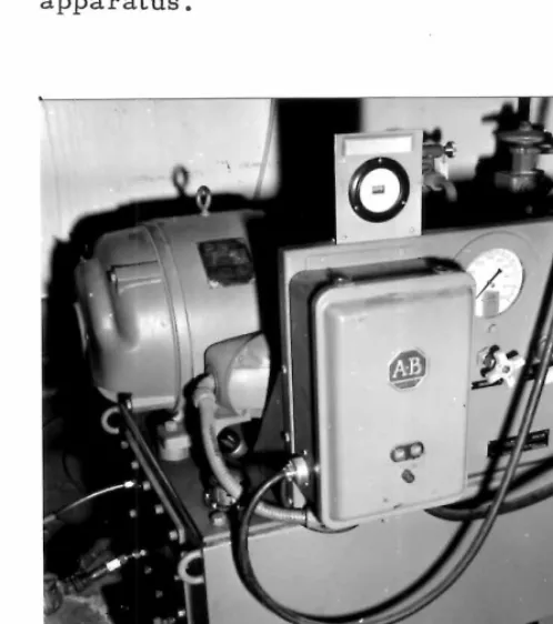
The model was made to oscillate hydraulically. A Dennison variable displacement pump supplied oil at 1250 psi for these experi-ments. The pump and oil reservoir are shown in Figure 3. This oil, controlled by a servo valve, causes a double-acting piston to move up and down in a cylinder.

The servo valve and actuating mechanism are shown in Figures 4 and 6. It was designed and built by Team Corporation of El Monte, California. Not pointed out in the figures are the position and

•

velocity transducers which sense the motion of the piston and provide feedback information to the servo controller. The position trans-ducer is a linear variable differential transformer (LVDT) and the velocity transducer is nothing more than a magnetized iron core inside a coil of wire. The voltage generated is proportional to the number of lines of force being cut per unit time and hence the velocity.

Co Servo Controller

The device which took the input signal, compared it with the feedback and generated the signal to the servo valve is called the servo controller. It was designed and built by the McFadden

Electronics Company of South Gate, California, and is Model 150A 0 It was designed to be operated with position, velocity or force

e

because this gave the best response in the frequency range of interest. D. Models and Attachment Fixtures

The models, shown in Figure 5, are two sharp-edged delta wings with apex angles of 15 and 30 degrees. They were fabricated from one-quarter inch aluminum plate and are both approximately one foot in length. Their bottom sides are both flat and a two-stage bevel, rounded by hand, was used on the top. This produced quite sharp edges. The effect of camber is negligible, particularly in light of the leading edge separation which occurs in all three types of flow (i.e., planing, fully wetted and ventilated).

Provision for running different angles of attack was accom-plished through spacers placed between the model and the force balance. This assures a simple rigid system in which the angle can be reset at will. It does not have the flexibility of a continuously variable device, but has proved very workable here.

E. Instrumentation

1. Lift and Pitching Moment Balance

The measurement of the unsteady lift and pitching moment forces was accomplished by a strain gage strut balance. That is, the balance is an extension of the support strut. The placement of the balance is shown in Figure 6. The balance was constructed so that

•

-16

-

was attached a conventional wire strain gage bridge. By summing the forces in the two vertical links the lift is obtained; by differencing them the pitching moment is obtained. It was found in static tests after the balance was constructed that the drag element had an

unacceptable amount of lift interaction and consequently this balance was not used for drag measurements but rather a new one was

designed. It is described in some detail in the next section. The lift and pitching moment balance is shown in Figure 7 before the installation of the strain gages. The wires for the bridges pass through a hole in the top of the balance, up through the center of the support strut and piston to a connector at the top of the oscillator. After the installation of the strain gages metal plates were soldered • to the sides of the balance for mechanical protection and to provide

support for the waterproofing which consisted of thin sheets of latex cemented around the outside of the balance. The balance was

slightly pressurized via the hole carrying the wires to prevent water from entering the balance in the event of a leak.

The balance is fairly rigid having no natural frequencies below 200 cps, but a dynamic calibration of both lift and pitching moment was provided at each of the operating frequencies to obviate the effect of a dynamic magnification factor. The calibration is discussed in more detail later.

2. Drag Balance

•

dynamic drag measurements are quite scarce a new balance was designed to measure drag only with the hope of isolating all other forces and moments and eliminating all interactions. _{The final} balance showed in extensive static tests that it did just that to the least count of our equipment.

The balance is shown in Figure 8. _{It consists of two over-} lapping side plates which are about 0.2 inch thick and very rigid, one of which is attached to the support strut and the other to the model. The side plates are connected to each other in turn by a system of flexures and an instrumented link to measure the drag force. This drag link is shown in Figure 9.

The flexure system consists of four thin metal sheets lying • in two vertical transverse planes. Each flexure is 0.8 inch high,

0.005 inch thick and 0.2 inch in the lateral direction. _{They were cut} from sheet stock and furnace brazed in position. _{They carry all loads} except drag for which they are comparatively flexible. _{The instru-} mented link carries most of the drag force providing high sensitivity. It is a flat bar approximately 0.3 inch high, 3 inches overall length and 0.050 inch thick except in the central instrumented portion where it is 0.030 inch thick. _{It is attached at the front to the grounded} side and at the back to the model side. _{This puts the link in tension.} Small "cut-outs" were machined into the link at each _{end just}

inboard of the attachments to prevent unwanted moments from getting to the instrumented section.

- 1 8 -

gages. Their placement on the gaged section was further planned to cancel any moments which might creep in. Temperature compensa-tion is also provided by gage matching but that is of little importance in this application.

Because the gages could not be in place during the brazing the balance was designed so that the drag link could be inserted through an opening in the trailing edge after brazing and fastened in place by dowel pins and cap screws through access holes in the side pieces. The opening in the trailing edge was filled with a brass plug to provide support for the waterproofing. This has the added advan-tage of easing maintenance should the gage fail. Waterproofing is provided as on the lift balance by thin latex sheets cemented to the outside of the balance.

The balance was designed so that it is sufficiently rigid in the drag direction (i.e., its natural frequency is above 600 cps with a model attached) so that it could be calibrated statically and the same factor used at all frequencies.

3. Voltage Supplies and Amplifiers

Figure 11 will be helpful in showing how the electronic equipment is patched together. The excitation voltages for the strain gage bridges were provided by a Microdot Power and Balance Unit PB-200A for each. They have provision for patching resistors on a conditioning board to approximately balance the bridge. A poten-tiometer was also _{provided for balance which was useful for nulling}

•

•

excitation voltage. A Microdot Voltage and Balance Monitor VB-300 was used to monitor the excitation voltages and to null the bridge output during steady operation.

The output of the strain gage bridges was fed through a series of Burr-Brown Model 1685 amplifiers. In the lift-pitching moment balance the outputs were summed and differenced in the first two amplifiers to produce lift and pitching moment. These outputs went to a selector switch so that only the signal being analyzed would be fed to two other amplifiers connected in series. The total gain was then 1000.

4. Return Signal Analyzer

•

The force signals and heaving velocity signals were analyzed in Boonshaft and Fuchs _{Model 711A Return Signal Analyzer}

(RSA). The signal being analyzed is compared internally to a signal of the same frequency as the command signal. A Fourier analysis is performed electronically and the components can be read out on meters or on an auxiliary voltmeter.

5. Variable Phase Low Frequency Oscillator

-20--

•

The output of the RSA was connected to a Non-linear

Systems Series 2900 Digital Voltmeter. This is an integrating meter and the integrating times most frequently used were one and ten seconds, the latter used if the data were unsteady.

7. Position and Velocity Transducers

The position and velocity transducers were mentioned earlier. The primary functions of the position transducer were to aid in the calibration of the velocity transducer and to provide static height stability in the servo controller. The velocity transducer provided the phase reference for the force data and was also used in

•

the normalization of the forces.

F. Support and Ventilation Struts

The support strut tying the model and force balance to the piston of the oscillator is a NAGA 0010 section of 10 percent thickness and 4 inch chord. It was designed to - minimize ventilation from the free surface. The force balances had similar contours to continue the strut profile to the model. The angle changing spacers were also contoured similarly.

•

arc welded at the leading and trailing edges. This was slipped over the support strut and attached to it above the balance. A means was provided to seal the upper end and air supply and pressure fittings were provided. The ventilation strut is shown in Figure 10.

G. Ventilation Measuring Apparatus 1. Air Supply Measurement

The air supplied to the cavity during the ventilating runs was measured by a Fischer-Porter flowrneter and the supply pressure was measured on a Heise Bordon tube pressure gage. The reduction of the data is discussed later.

2. Cavity Length Measurement

• The cavity length was measured with a tape rule held against the working section side. This method probably is not

accurate to less than an inch but considering the difficulty in defining the _{termination point for the cavity this accuracy was quite acceptable.}

3. Cavity Pressure Measurement

•

-22-

III. EXPERIMENTAL PROCEDURE A. Calibrations

1. Position Transducer

The position transducer was calibrated using a microscope attached to a lead screw and counter. The lead screw and counter were geared together so that the counter read directly in thousandths of an inch. The microscope could be set with the cross hairs aligned to a mark on the oscillator shaft; a number of position and voltage readings would then be made and the data least squares fit with a cubic polynomial. The linear term is the only one which is used since over the range covered in the velocity transducer calibration only the linear

•

term is important.

2. Velocity Transducer

The velocity transducer was calibrated using the position transducer since the motion was simple harmonic. At each of the frequencies used in the experiment the velocity and position signals were analyzed using the Return Signal Analyzer. Since for simple harmonic motion the velocity amplitude is just the angular frequency times the position amplitude, and since we know the position cali-bration factor, we can then infer the velocity calicali-bration factor.

3. Lift and Pitching Moment Balance

The lift and pitching moment balance was calibrated both statically and dynamically. Static tests were run to determine the electrical position of each of the force links and the excitation

•

voltages were chosen so that both of the lift gages (N

1 and N2) had the same output/unit force. This must be done, otherwise the balance will have a lift-pitching moment interaction.

The dynamic calibrations were done at each frequency because even though the balance's natural frequency was well above those used in the experiment this afforded an easy way to obviate errors due to dynamic response. A two piece calibration mass shown attached to the strut in Figure 10 was fabricated specifically for this task. The upper part, made of aluminum, was bolted to the strut at the model attachment holes. The bottom part, much heavier and fabricated of brass, was made so that it could be attached to the aluminum bar at any of six different positions to vary the longitudinal center of gravity • of the total live mass. Using Newton's second law and the

character-istics of simple harmonic motion the forces were inferred from knowing the mass and the velocity transducer output. By oscillating the mass at two different longitudinal positions (generally the end ones) the pitching moment calibration coefficients and the longitudinal electrical center were determined. This also allowed a check on the sensitivity of lift to pitching moment changes.

4. Drag Balance

The drag balance presented a much easier calibration problem. Because of its designed-in constant response over the test frequency range the calibration could be and was done statically. This consisted of bolting a fixture to the bottom of the balance and

.

-24- •

bags could be hung. The problem of assuring that the line was pulling in the drag direction was handled by levels on both the fixture and the line. Having only one load-carrying element in the drag direction no matching of outputs was required as in the "lift" balance, therefore the excitation voltage was changed to maintain a fixed calibration coefficient over the period of drag testing.

As a check for whipping of the strut the balance was oscillated with the tunnel dry and no sensible drag output was noted.

5. Return Signal Analyzer

The manner in which the force coefficients were normalized meant that the Return Signal Analyzer processed a signal in the

denominator as well as the numerator. This means that an absolute • _{calibration was not required (in fact, it was checked against an rms}

voltmeter and appeared to be within two percent of scale) but only variations from scale to scale. These relative coefficients were obtained using a signal from the Velocity Phase Low Frequency Oscillator and leap-frogging from scale to scale. Except for the two lowest scales they were within one percent of the ratio of scales so even had they not been accounted for, and they were, the effect would hardly have been noticed.

6. Air Supply Apparatus

•

The flow meter was a Fischer-Porter product with tube No. FP-3/4-27-G-10/80 for which a calibration curve was provided by the manufacturer. It was double-checked against another flow meter which had been previously calibrated and was within the five percent tolerance, over the working range, that these instruments are good for.

The supply pressure, which never exceeded 70 psi at the flow meter, was measured by a Heise gage No. H1665. This gage was checked with a dead weight tester and found to be within 0.1 psi from zero to ninety-five psi. This was the accuracy to which the gage could be read.

The cavity pressure was given by a water manometer less the • pressure drop in the ventilation strut. This pressure drop was

accounted for by running various air supply rates through the strut with the tunnel dry and calculating the relationship between pressure drop and mass flow rate. This drop was then subtracted from the apparent cavity pressure in the final data reduction.

B. Parameters Investigated

There are basically six parameters whose influence on the force coefficients was investigated. They are angle of attack,

aspect ratio, reduced frequency, submergence, oscillation amplitude and air supply rate. Not all combinations of the parameters were run due to the time involved, however representative checks were made where it was felt appropriate.

• -26-

depending on the type of flow. _{For instance, in the fully wetted runs}

angles of zero, six and twelve degrees were run for each of the

submergences. _{The planing runs, however, were done only at six}

and twelve degrees since proper planing cannot be established at zero

degrees. _{The ventilated runs were performed at twenty degrees}

angle of attack because this is near the lowest angle that the model could be fully ventilated under the test conditions.

In addition to the basic data runs, tests were done at minus six and minus twelve degrees with the model fully wetted and at the deepest submergence. This was done to give some justification to the assumptions that the camber and strut effects were small.

Two different models were used. _{They were both fabricated}

• _{from 0.250 inch aluminum plate and have sharp edges all around to}

insure flow separation. _{Both models were approximately one foot in}

length and had apex angles of 15 and 30 degrees. _{The aspect ratio}

of these two models is 0.526 and 1.071 respectively.

One of the most varied parameters in the tests was the

reduced frequency. In all of the runs except the ventilation tests the reduced frequency was the one varied, by means of the frequency,

having fixed the other variables. _{In addition to the fundamental}

influence _{of the reduced frequency on the force coefficients, various}

tunnel velocities were run to determine the effect of obtaining the reduced frequency by different frequency-velocity combinations ° This was done only at an angle of attack of twelve degrees, 30 0 model and at maximum submergence since this was thought to provide the

•

The effect of the free surface was investigated in the fully wetted tests by running the models at approximately two, six and ten inches submergence. These large submergence changes were

accomplished by inserting spacers between the box holding the hydraulic oscillator and the tunnel.

For the data reduction it was desirable to normalize the force coefficients with the heaving velocity but to do this it was necessary to establish that the effect on these coefficients of changing the

amplitude was negligible. Since it was impractical to do this at every combination of parameters the case of the 30 ° delta wing, 12 0 angle of attack, 0.83 chord submergence and 16.5 ft/sec tunnel velocity was chosen as at least representative if not a worst case. In the • planing runs the oscillation amplitude was more constrained by other

things to small values, consequently the effect was that it was not practical to measure but was thought to be very slight.

In the ventilation runs a whole new group of parameters was introduced. They are the air supply rate, the cavity length and the cavity pressure. These parameters are all directly related to each other so the situation is not quite as complicated as it sounds. The basic variable chosen was the air supply rate but the other data were also computed.

C. Data Runs

In this section we will be concerned with the actual steps of data gathering. For the most part the steps are the same for both

•

-28-

two in any particular run was the frequency whereas in the ventilation runs the air supply rate was varied.

Before the start of a run we must select and fix the following "variables":

1. Model

2. Angle of attack 3. Submergence

4. _{Oscillation amplitude (fully wetted)} 5. Tunnel velocity

At some time during the testing each combination of model and attachment fixtures must have its mass determined because the force due to the "live" mass and the acceleration must be accounted for to • _{determine the fluid mechanical forces.}

This was accomplished by assembling the model and fixtures as for a test and then with the tunnel dry the model would be oscillated and the live mass tare determined.

Having fixed the above parameters and with the tunnel full and operating at the chosen velocity but with the model stationary, the bridge excitation voltages are checked and the bridges balanced to limit the DC input to the RSA. _{With the static bridge outputs zeroed} the amplifiers are balanced. _{Now the model can be oscillated.}

•

•

0

-29-

this way a velocity reference is obtained. _{The force is applied to the} RSA. _{That part of the force signal observed on the channel previously} containing the velocity has the same phase as the velocity. _{The second} output channel gives the quadrature component of force.

In a typical data block zeros are taken for each channel with the input shorted. _{The heaving velocity is applied to the RSA and read.} The force signal is applied and each channel read. _{The input is again} shorted and zeros again taken. _{When using the "lift" balance, the} first force taken is the lift. _{After the second set of zeros another} velocity is taken and then the pitching moment. _{This routine is}

repeated again at constant frequency so that redundant lift and pitching moment readings are obtained with sets of zeros before and after each force reading. _{The data taking is similar for the drag balance except} that only one force is being read. _{This process is repeated at each of} the frequencies investigated.

The ventilation runs are similar in that the bridges and

amplifiers are balanced with the model stationary and the RSA outputs are zeroed with shorted input. _{The primary difference lies in that the} frequency is fixed not just for a "block" of data but for an entire

"run". _{The parameter varied within the run is the air supply rate.} D. Data Reduction

The data reduction was accomplished for the most part with the aid of an electronic digital computer. The repetition makes the job boring which encourages errors when done by hand. The computer is

•

-30-

IBM 7094 computer which is something like killing flies with a steam shovel but it was the only one of convenient accessibility.

The calibrations and data reduction are intimately tied together, consequently some overlap with the previous section on

calibrations must be expected. The equations defining the calibration coefficients and their use in the data reduction are presented here.

1. Force Coefficients

We will assume that the hydrofoil is performing a simple harmonic heaving motion. The vertical displacement transducer output is then given by a relation of the form

•

where y is the vertical displacement transducer output, F 1 the displacement calibration coefficient obtained as described previously and A is the amplitude. Feeding this displacement signal into the RSA we get (all RSA output signals will be denoted by tildes)

= C AF 1 ₍₂₎

where C is some constant associated with the Fourier analysis performed by the RSA.

Because the motion is simple harmonic the velocity transducer output can be written in the form

= F2 A o.) cos cot ₍₃₎

e

calibration factor

' F2 . The signal becomes, after processing by the RSA,

= F

2 C A co (4)

or substituting equation (2) into equation (4) we get

= F _{2 F} co• ₍₅₎

' 1 Solving equation (5) for F

2 shows us explicitly how we may obtain this calibration factor.

F 1 y — = —

F 2 (A)

(6)

• _{The acceleration is also directly related to the velocity and} since we know the value of the calibration mass we can use Newton's Second Law to infer the force output.

'2 F = - m F

3 A co sin cot (7)

This equation defines the lift force calibration factor F 3 and m is the calibration mass (toa1). The signal as processed by the RSA is

= - m F 3 C A co 2 . ₍₈₎

Substituting equation (4) into equation (8) the RSA output becomes

= - m F o.) ₍₉₎

•

and solving this expression for F 3 we get equation (10).

F

2 F

F₃ = - — — ₍₁₀₎

The rms dynamic lift is then related to the RSA output signal through the factor F

3*

. = L . • F ₍₁₁₎

r, 1 r, 1 5

The subscripts r and i have been used to denote the force components in-phase with the apparent change of angle of attack and 90 ° out of phase.

The apparent change of angle of attack is given by

•

U P

2 (12)

The in-phase lift coefficient is then defined by and calculated using equation (13).

L

r 2 F_2r

C

La-

1

3 .Sr (13)

The quadrature lift coefficient is then defined by and calculated using equation (14).

L. _{2 F}

2 ( -

1 m F 3

C L

co 1

a pUA F3 F2 )

(14) i PU

A Et

•

The second term in parentheses in equation (14) represents the force due to the acceleration of the model's mass and the live mass of the balance. The total live mass is m .

The pitching moment calibration is similar. The calibration mass m has its center of gravity at a distance _{from the}

electrical center of the balance. This offset causes a moment as the mass is accelerated vertically. The moment signal can be expressed in the form

t

M = F

4A c 2

o sin cot . ₍₁₅₎

This equation defines the pitching moment calibration factor F 4 and the processed signal can be expressed as

•

₁

_■

71 = m F 4C A

'

co2 . ₍₁₆₎

Substituting equation (4) into equation (16) and solving for the calibration factor F

4 we get F

2 F

4 = m P CJ (17)

The rms dynamic pitching moment is related to the RSA output signal through the factor F 4 .

1

■

4 (18)

1", 1 r, 1

-34-

M

r 2F2 Mr

M-

PU 1 2

Acce

(19) r

-2-

The quadrature pitching moment coefficient is defined by and calculated using equation (20).

M.

2

c

m

_ -

a 1

na .e F

m

1 4(')

PU2 Ac =

pU A F4 c F

2

(20)

The distance of the total live mass from the electrical center of the balance is / and m is as for the lift. The pitching moments as given above are for moments about the electrical center of the balance. To obtain moments about a parallel axis through the model • _{planform's centroid we must have drag data.}

The drag is reduced in much the same way. The drag calibration factor is obtained statically and is the same for all frequencies. Also, because the motion is perpendicular to the

direction that the force is being measured there is no live mass tare. The drag force is related to the RSA output by

. =

5 (21)

r, r,

and the drag _{coefficients are given by}

D. 2 F

2

i5

.

r, 1 I', 1

C

a- - 1 2 - pU A F • (22)

5 -:-

—₂ PU A a _Y

2. Ventilation Parameters

The additional data taken during the ventilation runs were reduced to dimensionless parameters as follows.

The cavity length was measured with an ordinary rule and the number divided by the model chord length to produce a dimension-less cavity length.

The air supply rate was measured with a Fischer-Porter flow meter and the supply rate reduced to standard cubic feet per second using calibration information provided by the manufacturer. An air supply coefficient was defined as

•

C

This has the meaning of a column of air of cross-sectional area equal to the projected frontal area of the foil and moving at free stream velocity.

The ventilation number is analogous to the _{cavitation number} and is defined by

Pco pc v = 1 ,2

7

The cavity pressure was measured by a manometer connected to the ventilation strut. The pressure drop in the strut was calibrated as a function of the air flow rate so that the cavity pressure reading could be adjusted accordingly.

.

-36-

IV. A THEORY OF UNSTEADY PLANING OF SLENDER BODIES AT SMALL ANGLES OF ATTACK

A. Preliminary Remarks

We digress somewhat here to develop some theoretical

results so that they can be referenced in the course of discussing the experimental data. As was mentioned in Section I Tulin (30) has previously presented a theory for steady planing of slender bodies at small angles of attack. It is unfortunate that the paper containing Tulin's efforts has quite a few errors. Some of these are algebraic; others are perhaps conceptual. The paper nevertheless contains an interesting approach to the problem and the method used is basically correct.

The purpose of this section is two-fold. It is intended that Tulin's original problem be corrected. It is also intended that the problem be extended to unsteady planing and it is shown how the unsteadiness affects the validity of the approach. The specific cases of uncambe red delta wings at rest and oscillating in heave are treated in detail.

B. The

_{Coordinate System}

_{Bernoulli Equation}

The coordinate system used for the solution of this problem is shown in Figure 12. It is fixed to the foil with its origin at the foil's apex. The x-axis passes through the mid-point of the trailing

•

may have a small amount of camber but is assumed to be unyawed. Neglecting the effect of gravity the equation of motion of the fluid in this frame of reference is given by:

DI -Z.. 1

vb =

T

The term v

b ' not usually encountered in steady problems, is required because Newton's Second Law must be applied in an inertial reference frame. This term represents the acceleration of the

previously defined coordinate system with respect to an inertial one. The velocity of any fluid particle with respect to the

coordinate system of Figure 12 is q . This velocity is expressed

•

the velocity.

= ₍₂₄₎

Using this definition of .1, we can re-write equation (23).

1p

V Pt +

2- (v10) +

It should be noted that in the above equation motions normal to the free stream have been assumed. We can integrate equation (25) to get

1 p

The function B(t) is often called the Bernoulli constant since in steady problems it is a constant. Here it may be a function of time.

At infinity the velocity potential tt is given by

= (U cos« + v

b sin a )x + (U sin a - v_b cos a )y (27) co

From this condition on the potential at infinity we get upon substitution into equation (26) the value of B(t) .

1 B(t) = L

pc° — + — 1

(U ccs + v 2

b sin a ) + (U sin a - v_b cos a )2 2

(28)

By subtracting the potential at infinity we can define a new "perturbation" potential as in equation (29).

= - ₍₂₉₎

oo

Re-writing equation (26) in terms of the new potential c we get the exact unsteady Bernoulli equation for this problem.

1 _{2 1}

+ (

9

b sina ) + . 2. ( + U s in a - vb cos a )2

t c x

1 2 p 1

+ (

9 ) + — = — (

1 _co

•

9-

C. Laplace's Equation and The Boundary Conditions

Although it has not been stated we are taking the fluid to be incompressible and inviscid. The condition of incompressibility simplifies the continuity equation and the irrotation.ality following from the inviscid assumption allows us to write the velocity as the gradient of a scalar potential. The equation then that the velocity potential must satisfy is the well known Laplace's equation (31).

'72 (x, y, z; t) = 0 ₍₃₁₎

It is easily shown that the perturbation potential also satisfies the same equation.

• _{The boundary conditions on the perturbation potential will now} be constructed. From its definition the perturbation potential is seen to vanish at infinity. On the foil we have the condition that the flow must be tangent to the boundary, which gives:

/ =

y x yo (32)

where y o (x) is the camber function and the prime denotes differen-tiation with respect to its spatial argument. Equation (32) can be re-written as shown below.

= Yo

•

-40-

This boundary condition on the foil is exact. The boundary conditions on the free surface require some approximations. They will be

discussed in the next section. D. Approximations

From this point on we will assume that we are treating a "slender" body. What we mean by slender will become clear as the approximations are made. If we can assume as a result of this slenderness that q, <<

' it can then be neglected in

xx _YY z z

Laplace's equation and x becomes a parameter entering the problem only through the boundary conditions and the potential is not affected by conditions upstream. Laplace's equation can now be written as

v z

The problem has been reduced to a two dimensional boundary value problem in the so-called "cross-flow" plane.

We can also simplify the boundary condition on the foil under the assumptions:

1) a << 1 so that sin a a and cos a = 1 2) cp

x « U and 3) a vb « U. Equation (33) then becomes

4, L. 99 _{+ U a - vb U y}

or we can re-write this as

•

•

We have still to satisfy boundary conditions on the free

surface. The nature of the problem dictates that we should have free stream pressure everywhere on the free surface. _{The position of the} free surface, not known a priori, will be taken to lie along the z-axis. In the actual case, sketched in Figure 15, the free surface boundary is at y = a x at infinite distances from the foil and acquires a

complicated shape near the foil. _{The approximation that the boundary} conditions can be applied to the z-axis is necessary to keep the

problem tractable. _{Figure 14 presents a photograph of a 30 0 apex} angle delta wing planing at a small angle of attack. _{The spray can be} seen. _{Because of the difficulty of determining the shape of the spray} and the flow in the spray region, the spray will be represeAted as a • singularity. The separation of the tips of the spray depends on the

static height of the apex above the free surface, a slight amount of which will exist in any real situation.

As is shown in Figure 13 the spray singularity is taken at z = b

1 (i.e., = b). Outside of this point the flow is assumed to be undisturbed or rather that q)

z = 0 for I z I > b 1 and since

so = 0 at infinity, ci? = 0 for I z I > b

I also.

In the region between the leading edge, z = a(x) and

z = b

l we must determine a velocity boundary condition which at least approximates the pressure condition. _{This will be our next} concern.

•

(00 (y, z; x, t) = a(x) f t) (36)

The coordinates are given by:

Ti = —Y_a and = — _{a •} (37)

The derivatives of co expressed in terms of f and appropriate coordinates are given below.

x = ax (f - rif ₁ - f)

=

(38)

•

t = a(x) f1

On the foil and in the region near the leading edge the pressure equation becomes

2 = - U(P

x - —2 (U y o ) - —2 (50z)

1

+ (uct - v

b) 2

(39)

where the (92 x)

2

term has been neglected along with the assumptions following from the smallness of a • Replacing derivatives of (P by the appropriate functions of f and setting p = p c° we get that at the

.

'2 - 2U a

x (f - - (U y o ) - (f) 2

+ (U a -

2

- 2a(x) f

t = 0 (40)

We will now estimate the value of each term in this equation so that some of them can be dispensed with. Near the leading edge

-1- 1. Taking the distance from the leading edge to b to be _E and assuming f is approximately constant in that region we get that f(1)-; - cf (1) near the leading edge. Taking Ua

x— (1), U y

o 0 (6 ), U a —

er(

er (

)

2 •

1+ 0 = 2 U a

x (1

+

62 1

I - (UY )

2

- (f )2

62 k (52

+ (U - vb )2 + 2a(x)ft ₍₄₁₎

The reduced frequency has been denoted by k. The order of the last term in the above equation has not been shown yet. It will be shown later when c is calculated. Since we will seek a quasi-steady solution of this problem we can reasonably neglect this term until a time when the proper restrictions on its importance can be shown. Keeping only terms of

_tY

•

Conditions on f have now been specified along the entire _-axis. They are shown on Figure 13.

E. The Solution of the _{Boundary Value Problem}

The boundary value problem is seen to be, except for the unsteady parts, identical with Tulin's. The method of solution pro-posed by him and indeed part of his solution are used more or less directly. It is intended that the confusion in his paper has been removed in this solution.

The specified boundary conditions may be satisfied by a distribution of vorticity of strength 'Y t) along the -axis between -b(x, t) and +b(x, t).

1 _{(r,, t) d}

=

J (, _

-b

We can also re-write equation (43) below since _{y( t) =}

2f (-0, ; t).

-1 , , 1

i

i

Trf (0 = 1 _(:)

/1 i

- b ( - )

b

+ 1._I'

. f 00 ci

( - 0 (44)

We can apply the known conditions _{on f and f , namely}

= vb +

•

f (e) =Ua

x Sgn (e) for 1 <j < b •

Equation (44) then becomes the following where the only unknown is f for I e I <1 .

-1 Try = - 2Ua

x

f

dr,

- + 2 U ax

f

e -

-b

1

i

foo

+

-1

izi (45)

i

Re-writing this in the form of the conventional airfoil equation we have the following:

1 f

=

e -

-1 ,

- 21Ja

f

dr

x ( -

f

1 -b

for I e I <1

The formal solution of this equation can be found in Tricomi (32) and is taken from Tulin's work in the form given below.

-46-

•

4 (t)

1 _{1 - E.}2

2

_

TI

1

1

1

t

,

b -b

dT

-2a

f

f

d

X ( t - T ) + 2aX - T )

1 _-1

The vortex sheet limit b is determined later to make f (1) bounded.

If we combine integrations equation (46) becomes

1

f

₁

Tr a 2a

2

f

U x _{- 7)}

1T -

-1

y

+ 2a

x

f

1

1

i_

t)(

-b -1

Using the following identities:

I 1 1

1

- 7)

_

(t - T) ( - t )

+

]

fli 1

q - 0 d' -- r - Tr t for 1 I < 1 -1

1

1

₂

•

_{f 1}

, _ ,

, _

Ir.( - T - T T < -1 1

11 2 . - 1 ) 2 t

Tr ( - T T AIT - 1 ) T > 1

-

(46)

•

the following equations can be shown to be true:

_

a fb r

f,(0

=

117 2

j

u

d

Tr2

11 1 - e

1

_

171

T T

- 1

1-2a C1T

X

f

-1

+

-

-b

T)

f & (0

_ 1 1 _Dv_ + 47 ax

f

2 1 dT

}

(49)

U

111 - 2 \

1

0

With the substitution 111 - 2l tan

0

1:2-7-TI.

7

for b2 = 1 (i. e.,

E << 1 )

f ( ₁

—4 a b 2 - 1 U

1 - 11- X

1 b2 -1 - 1 - e tan -

- < 1

(50) 1

To keep f (1) bounded b must have a particular value; namely,

•

-48-

If we write b as 1 + E and take

E << 1

Tr

E =

32 U a

x _{) 2}

2

Tr Vb UY 0 ) 2

U a x

(53)

Previously we have assumed that Ua x ,

(1), vb , 6)- (,) ,

Uyo ,..,& ( a) and U a— _{(6) where 6 << 1 . From equation (53)} then we get directly that

E

(

•

_E

It was stated without proof in equation (41) that the last term of the equation was (k 62_{). This will now be shown. The term is given} below. It has been assumed f _{is constant in the region 1 < < b} thereby neglecting any waves, therefore:

-2a(x) f

t = 2a(x) f (54)

We can evaluate

E

2 (v + - U )

TV

c = 16

(U ax)2 Vb

Assuming simple harmonic motion for vb we get I i71D 1 = I, and a(x) is limited to c a

•

Substituting this into equation (54) we get the following estimate for the order of that term.

Tr 2 (vb U3ro U")

- 2a(x) f t — 2(ca x )(2Ua)-17 x

(Ua)x 2 c")vb

- ( 1(6 2 ) (55)

We may conclude then that for k

EY

Substituting in the required value of b we get the final solution for f .

•

f(°

₌

a x

We can also express this in unreduced coordinates.

Ua

q)_z -

- 4 a _Tr tan -1 L x _{for IzI < a (57)} x a

11 1 - (z/a) 2

This is the solution for so_z as given by Tulin.

F. The Calculation of Forces

-50-

a

dN

_f

[ p (0, z; x, t) - p oz) dz dx

-a

Using equation (39) this can be re-written as shown below.

a dN

= 1

I

f

-a

1

- 2- (U a - v

b) 2

clz

The first term of the above integral is evaluated using the relation:

410

,(0, z; x, t) =

a(1+ C)

a

761

= - 2 aEUa

x + f (0, x, t) d. a

And by an application of Leibnitz' rule we get

a _a

f

f

-a _-a

+ 4 a EU a x

2 •

(58)

(59)

(60)