Munich Personal RePEc Archive
The Role of Renewable Energy
Consumption and Trade: Environmental
Kuznets Curve Analysis for Sub-Saharan
Africa Countries
Ben Jebli, Mehdi and Ben Youssef, Slim and Ozturk, Ilhan
Manouba University, ESC de Tunis, LAREQUAD, Tunisia,
LAREQUAD FSEGT, University of Tunis El Manar, Tunisia, Cag
University, Faculty of Economics and Business, Turkey
7 March 2014
Online at
https://mpra.ub.uni-muenchen.de/54300/
1
The Role of Renewable Energy Consumption and Trade: Environmental
Kuznets Curve Analysis for Sub-Saharan Africa Countries
Mehdi Ben Jebli
LAREQUAD & FSEGT, University of Tunis El Manar, Tunisia. University of Jendouba, ISI du Kef, Tunisia.
benjebli.mehdi@gmail.com
Slim Ben Youssef
Manouba University, ESC de Tunis, Tunisia.
LAREQUAD & FSEGT, University of Tunis El Manar, Tunisia.
slim.benyoussef@gnet.tn
Ilhan Ozturk
Cag University, Faculty of Economics and Business, 33800, Mersin, Turkey. Tel: +90 324 6514828,
Email: ilhanozturk@cag.edu.tr
First version: March 7, 2014
Abstract: Based on the Environmental Kuznets Curve (EKC) hypothesis, this paper
uses panel cointegration techniques to investigate the short and the long-run relationship between CO2 emissions, economic growth, renewable energy consumption and trade openness for a panel of 24 Sub-Saharan Africa countries over the period 1980-2010. The validity of the EKC hypothesis has not been supported for these countries. Short-run Granger causality results reveal that there is a bidirectional causality between emissions and economic growth; bidirectional causality between emissions and real exports; unidirectional causality from real imports to emissions; and unidirectional causality runs from trade (exports or imports) to renewable energy consumption. There is an indirect short-run causality running from emissions to renewable energy and an indirect short-run causality from GDP to renewable energy. In the long-run, the error correction term is statistically significant for emissions, renewable energy consumption and trade openness. The long-run estimates suggest that real GDP per capita and real imports per capita both have a negative and statistically significant impact on per capita CO2 emissions. The impact of the square of real GDP per capita and real exports per capita are both positive and statistically significant on per capita CO2 emissions. For the model with imports, renewable energy consumption per capita has a positive impact on per capita emissions. One policy recommendation is that Sub-Saharan countries should expand their trade exchanges particularly with developed countries and try to maximize their benefit from technology transfer generated by such trade relations as this increases their renewable energy consumption.
Keywords: Environmental Kuznets Curve;Renewable electricity consumption; International
trade; Panel cointegration; Sub-Sahara.
2 1. Introduction
The electricity access in Sub-Saharan Africa is the lowest in the world. According to the report of the United Nations Environment Programme (UNEP, 2012), the region knew a considerable growth of 70% in the electricity production which is translated by an annual average growth rate of 6% for the whole region. The growth of renewable energies was so strong recently. The total production of electricity coming from renewable energies is increasing by 72% from 1998 to 2008. However, the renewable electricity generation increased from 45 to 78 terawatt per year. This result means that 66% of all new electricity produced in sub-Saharan Africa after 1998 comes from renewable sources.
There is a significant potential in Africa and particularly the Sub-Saharan countries for the use of renewable energy sources (solar, wind, water, geothermal, hydropower, tides, waves…). Although the amount of energy sources in the region is very large, the economic and social development indicators provide that these countries still the poorest in the world. Moreover, the use of renewable energy has not been seriously exploited because of the limit policy interest and investment levels. Mauritius, South Africa and Ghana are cited among Sub-Saharan countries to make-up a significant steps in increasing their potential in the consumption of renewable energy (Bekker et al. 2008).
Let notice that there are areas in Africa where solar energy potential can be considered very interesting. The solar energy can supply an alternative of electrification adapted to numerous rural localities isolated geographically in the sub-Saharan region. Unfortunately, there are very few initiatives for the exploitation of the solar energy in sub-Saharan Africa. However, in Zimbabwe, there is an effort has concerted to use the systems of solar energy for the production decentralized by electricity in the rural zones within the framework of the Global Environmental Facility (GEF). Besides the financial support limited by the government, most of the projects of solar energy on community base are sponsored or supported by the donor agencies (Suberu et al., 2013).
Demirbas et al. (2009) suggest that the global potential of bioelectricity increased from 104.8 to 183.4 TWh, with an average growth rate of more than 5.8%, between 1995 and 2005. However, biomass power is considered as the largest renewable resources in Sub-Saharan countries. It seems that 90% of people in sub-Sub-Saharan Africa use biomass (wood or residues) for cooking and heating and 60% of African women living in rural areas have to deal with the scarcity of supply of firewood.
Compared to the other renewable resources (solar, biomass and hydroelectric…), the use of wind power is rather low in Sub-Saharan regions. According to the Global Energy Network Institute (GENI, 2013), the best winds in Africa are found in the north of the continent and to its extreme east, west and south. Egypt is the most advanced in exploiting wind energy, with over 15 MWe installed capacity and there is also much additional potential. Based on the wind energy map and taking into accounts the climatological aspects, four southern African countries are identified to have the best wind resource are South Africa, Lesotho, Madagascar and Mauritius.
Hydropower is the main source of renewable energy in the worldwide. It represents 16% of the global power. More than 90% the untapped economically feasible potential is in developing countries, mainly in sub-Saharan Africa, South Asia and East and Latin America. Africa exploits only 8% of its hydropower potential. Kaygusuz (2011) mentioned that for many countries in Africa and South Asia, regional hydropower trade could provide the energy supply at a lower cost with zero carbon emissions. But the absence of political will and faith and concerns about energy security constrain such trade.
3
studies have not examined the impact of international trade and renewable energy consumption on emissions and especially in Sub-Saharan countries. We evaluate the current paper as a complementary to the one who was published by Ben Aïssa et al. (2014). For a panel of 11 African countries, Ben Aïssa et al. (2014) examine the dynamic interaction between economic growth, renewable energy consumption and trade using a production model. The finding of their analysis reveals that no dynamic causal relationship exists between renewable energy consumption and any other variables in both the short and the long-run. Also, because of the low rate of renewable energy in Africa countries, it is contributing to the increase of output is either very weak or not significant.
The paper is organized as follows: Section 2 gives literature review; Section 3 provides data information, modeling and methodology; Section 4 presents empirical results and Section 5 deals with conclusion and policy implications.
2. Literature Review
The short-run and the long-run dynamic relationship between CO2 emissions, economic growth, renewable energy consumption, and trade openness is one of the most important studies that we try to explore for a sample of Sub-Saharan countries.
Recently, numerous empirical analysis studies prove that renewable energy consumption plays a vital role for combating global warming (e.g. Apergis et al., 2010 and Sadorsky, 2009a) and the increase of output (e.g. Apergis and Payne, 2010a, 2010b, 2011, 2012; Menegaki, 2011, Ocal and Aslan, 2013; Sadorsky, 2009). The results from these papers are different depending on the selected data, period, and methodology used for the empirical analysis (ARDL, panel cointegration, variance decomposition, Toda-Yamamoto, panel random effect model, panel error correction model). The direction of causalities come from these papers have been established using various techniques such as Granger causality, and Toda-Yamamoto causality. However, some of them suggest the existence of bidirectional causality between renewable energy consumption and economic growth. It means that these studies support thefeedback hypothesis. Thus, this hypothesis exposes that any increase in the share of renewable energy in total energy use will increase output and it supports that any increase in economic growth (real GDP) causes an increase in renewable energy consumption. The Toda-Yamamoto causality test results in Ocal and Aslan (2013) show that there is a unidirectional causality running from economic growth to renewable energy consumption. This result supports the conservation hypothesis which argues that any change in economic growth will change renewable energy consumption but otherwise is not supported.For the United States, only one causal relationship running from biomass-waste-derived energy consumption to real GDP has been founded in Yildirim et al. (2012) during the period 1949-2010. This findings support the growth hypothesis which means that any reduction in the consumption of renewable energy will affect economic growth. Menegaki (2011) investigates the causality between renewable energy consumption and economic growth for a panel of twenty seven European countries during the period 1997-2007. The neutrality hypothesis is supported in the empirical test. However, the result involves that no causality between economic growth and renewable energy consumption.
4
causality tests reveal that there is bidirectional causality between renewable energy consumption and economic growth in the short-run and long run relationship. Furthermore, Granger causality indicates that nuclear energy consumption contributes to the reduction of CO2 emissions while renewable energy consumption does not.
Another group of papers discuss the dynamic relationship between output, energy consumption (renewable or total energy use) and trade openness (e.g. Ben Aissa et al., 2014; Sadorsky, 2012). The results from these two studies are not identical and the directions of the dynamic causalities are different. However, the finding in Ben Aissa et al. (2014) indicates that no causal relationship between renewable energy consumption and economic growth or between renewable energy consumption and trade in the short and long-run whereas the paper of Sadorsky (2012) suggest, for a panel of 7 South American countries, that short-run shows a bidirectional causality between energy consumption and exports, output and exports and output and imports and unidirectional short-run relationship from energy consumption to imports. In the long-run, the result indicates a causal relationship between trade and energy consumption. Thus, these two studies recommend that more trade openness could be a good policy to increase output.
A numerous empirical studies discussed the causal relationship between environmental indicators (CO2, SO2…), economic growth, energy consumption and/or trade (e.g. Acaravci and Ozturk, 2010; Arouri et al. 2012; Haggar, 2012; Jaunky, 2011; Ozcan, 2013) for the heterogeneous panel studies and Ang (2007), Halicioglu (2009), Jalil and Mahmud (2009), Ozturk and Acaravci (2010), Jayanthakumaran et al. (2012) for cross-sectional studies. Given that the purpose of our analysis is not to cite all the existing review but we will discuss only some studies.
5
are explained by energy consumption, income and trade, and the second form is that carbon emissions, energy consumption, and trade are determinants of income. From the first form which respects the EKC hypothesis, the empirical results suggest that income is the most significant variable followed by energy consumption and trade.
Ozturk and Uddin (2012) investigate the long-run Granger causality relationship between energy consumption, carbon dioxide emission and economic growth in India over the period 1971-2007. The augmented Dickey–Fuller test (ADF), Phillips-Perron test (PP) and KPSS test are used to test for Granger causality in cointegration models which take account of the stochastic properties of the variables. Feedback causal relationship between energy consumption and economic growth is found in India. The value of the error correction term confirms the expected convergence process in the long-run for carbon emissions and growth in India which implies that emission reduction policies will hurt economic growth in India if there are no supplementary policies which seek to modify this causal relationship. Jayanthakumaran et al. (2012) test the long- and short-run relationships between economic growth, trade, energy use and endogenously determined structural breaks for 1971-2007 period using the ARDL bounds approach for China and India. They found that CO2 emissions in China were influenced by per capita income, structural changes and energy consumption.A similar causal connection cannot be established for India.
3. Data, Specification Model and Methodology 3.1. Data
The data set is a balanced panel of 24 Sub-Saharan countries1 over the period 1980-2010 and includes annual data on per capita CO2 emissions, per capita real GDP, square of per capita real GDP, per capita renewable energy consumption, per capita real exports and per capita real imports. The time series data are selected to get the maximum number of observations depending on the availability of the data and time period. The CO2 emission per capita is measured in metric tons per capita. Real gross domestic product per capita (GDP, output) is measured in constant 2005 US dollars. Exports and imports are both defined as merchandise exports and merchandise measured in current US dollars. These variables are transformed from the current value to the real one by dividing them by the consumer price index (pc) and then divided by the population to get the per capita unit. The renewable energy consumption is measured in billion kilowatt hours and then divided by the population to get the per unit. It comprises electricity coming from geothermal, solar, wind, tide and wave, biomass and waste, and hydroelectric. Data on per capita CO2 emissions, per capita real GDP, merchandise exports and merchandise imports are obtained from the World Bank Development Indicators online database (WDI, 2013). Data on renewable energy consumption are obtained from the U.S. Energy Information Administration (2013) online database. Data on (pc) and population (in thousand) are obtained from the Penn World Tables version 7.1 (Heston et al. 2012). All variables are transformed to the natural logarithms form. Our estimations are done using Eviews 7.0 software.
3.2. Specification model
Our specification model is based on the EKC hypothesis and follows the methodology of Ang (2007), Halicioglu (2009) and Jayanthakumaran et al. (2012) for cross-sectional series and by Haggar (2012) and Narayan and Narayan (2010) for heterogeneous panel. The multivariate framework is established to investigate the long-run relationship between CO2 emissions per capita (e), per capita real GDP (y), the square of per capita real GDP (y2), per capita
1
6
renewable energy consumption (re) and per capita trade openness (o)2 (exports or imports) in two separate specification models. The first model includes per capita real exports (ex) and the second includes per capita real imports (im).
The log linear quadratic form is specified as follows:
2
0 1 2 3 4
it i i i it i it i it i it it
e =α +βt+α y +α y +α re +α o +ε (1)
where i=1,..., 24and t=1980,..., 2010 indicate the country and time series, respectively. α0i and βi denotes the country specific fixed effects and deterministic trends.εit indicate the estimated residual which characterize deviations from the long-run equilibrium. With respect to the EKC hypothesis, the sign of α1i is expected to be positive whereas the sign of α2i is expected to be negative. It means that an increase in per capita real GDP would lead to an increase in per capita CO2 emissions, whereas an increase in per capita square of real GDP would lead to a decrease in per capita CO2 emissions. The sign of α3i is expected to be mixed and depending on the specific economic development of the selected countries. With respect to renewable energy, we expect that the sign of α4i is negative if the share of renewable energy used is high enough and the industrial sectors use the clean technology for production; but it could be positive if the share of renewable energy is rather low and the technology used for production is polluting. The sign of α4i is expected to be mixed and also depends on the economic development of the selected countries. According to the discussing studies of Grossman and Krueger (1995); Halicioglu (2009) and Shahbaz et al., (2012), the sign of trade openness slope parameter is positive if the dirty industries of developing economies are producing with heavy share of CO2 emissions.
3.3. Methodology
We use panel cointegration test to check for the short and long-run relationship between emissions, economic growth, renewable energy consumption and trade openness for a panel of 24 Sub-Saharan countries over the period 1980-2010. Our empirical analysis follows five steps: i) we start through testing the panel integration order of each variable, ii) we look for long-term cointegration between variables, iii) we estimate the long-run relationships between variables using OLS and fully modified OLS (FMOLS), iv) we examine the causality between variables using Engle and Granger (1987) approach and v) concludes.
4. Empirical Results 4.1. Unit root tests
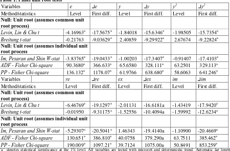
Fives panel unit root tests are used in this empirical analysis. Breitung (2000), Levin et al. (2002), Im et al. (2003), tests of Fisher use Augmented Dickey and Fuller (ADF) (1979), and Phillips and Perron (1988). These tests are composed on two groups: the first group of tests includes t-statistic of the Breitung (2000) and LLC’s test (Levin et al., 2002). These tests assume a common unit root process across the cross-section for the null of a unit root. The second group of tests includes IPS-W-statistic (Im et al., 2003); ADF-Fisher Chi-square (Dickey Fuller, 1979) and PP-Fisher Chi-square (Phillips and Perron, 1988). These tests assume an individual unit root process across the cross-section. For all these tests, the null hypothesis is that there is a unit root and the alternative hypothesis is that there is no unit root. Panel unit root is tested using intercept and deterministic trend for all variables.
The results from the panel unit root tests are reported in Table 1 and indicate that all variables are stationary after the first difference. However, for real GDP per capita, square of real GDP, per capita real exports per capita and real imports per capita, all tests suggest that
2
7
these variables have a unit root at level but they become stationary after the first different. For per capita CO2 emissions and per capita renewable energy consumption only Breitung (2000) reveal that these variables are non-stationary at level but stationary after the first difference. Finally, according to the t-statistic of Breitung (2000), we conclude that all analysis variables have a unit root at level and become stationary after the first difference.
Table 1. Panel unit root tests
Variables e e y y y2 y2
Method/statistics Level First diff. Level First diff. Level First diff.
Null: Unit root (assumes common unit root process)
Levin, Lin & Chu t -4.16963a -17.5675a -1.84018 -15.6346a -1.98505 -15.7354a
Breitung t-stat -0.21763 -9.03629a 2.40859 -9.29922a 2.67674 -9.22824a
Null: Unit root (assumes individual unit root process
Im, Pesaran and Shin W-stat -3.83765a -19.0433a -1.00203 -17.3407a -0.91407 -17.4103a
ADF - Fisher Chi-square 90.3680a 366.633a 65.6580 328.111a 63.2501 329.113a
PP - Fisher Chi-square 136.132a 1178.07a 61.9766 638.680a 58.6063 641.246a
Variables re re ex ex im im
Method/statistics Level First diff. Level First diff. Level First diff.
Null: Unit root (assumes common unit root process)
Levin, Lin & Chu t -6.46769a -19.1297a -2.01131 -16.6181a -1.43419 -17.9420a
Breitung t-stat -0.01950 -9.31175a -1.52556 -10.4094a -1.59992 -12.6234a
Null: Unit root (assumes individual unit root process
Im, Pesaran and Shin W-stat -5.29307a -20.5041a 1.46343 -19.4140a -1.10900 -20.4669a
ADF - Fisher Chi-square 130.651a 386.810a 40.0758 379.290a 63.7511 385.462a
PP - Fisher Chi-square 190.009a 1097.21a 39.7124 1075.00a 50.8491 853.259a
“a” denotes statistical significance at the 1% level. All variables are tested with intercept and deterministic trend. Automatic lag length selection based on SIC (Schwarz Information Criteria).
4.2. Panel cointegration tests
We use the Pedroni’s (1999, 2004) cointegration tests to ckech for the long-run relarionship between variables. Pedroni (2004) proposes seven statistics distributed on two sets of cointegration tests. The first set comprises four panel statistics and includes v-statistic, rho-statistic, PP-statistic and ADF-statistic. These statistics are classified on the within-dimension and take into account common autoregressive coefficients across countries. The second set comprises three group statistics and includes rho-statistic, PP-statistic, and ADF statistic. These tests are classified on the between-dimension and are based on the individual autoregressive coefficients for each country in the panel. The null hypothesis is that there is no cointegration (H0:ρi =1 ), whereas the alternative hypothesis is that there is cointegration between variables. Panel cointegration tests of Pedroni (1999, 2004) are based on the residual of Eq. (1). The estimated residuals are defined as follows:
1
ˆit iˆit wit
[image:8.595.72.522.169.464.2]ε =ρ ε − + (2)
8
among the three statistics used of the between-dimension reject the null hypothesis of no cointegration at the 1% significance level. Therefore, four tests among seven confirm the existence of long-term cointegration between the variables.
Table 2. Panel cointegration tests (e=f(y, y2, re, ex))
Alternative hypothesis: common AR coefs. (within-dimension)
Weighted
Statistic Prob. Statistic Prob.
Panel v-Statistic -1.414328 0.9214 -3.903998 1.0000 Panel rho-Statistic 0.472262 0.6816 1.548502 0.9392 Panel PP-Statistic -5.623830 0.0000*** -5.743216 0.0000*** Panel ADF-Statistic -6.798875 0.0000*** -7.541510 0.0000*** Alternative hypothesis: individual AR coefs. (between-dimension)
Statistic Prob.
Group rho-Statistic 2.362836 0.9909 Group PP-Statistic -6.546602 0.0000***
Group ADF-Statistic -6.060808 0.0000***
*** indicates statistical significance at the 1% level. The null hypothesis is that there is no cointegration among variables whereas alternative hypothesis is that there is cointegration. Lag length selection based on SIC (automatically) with a max lag of 5.
Table 3 reports the Pedroni (1999, 2004)’s cointegration results for the model with imports. As shown for the model with exports, the results of cointegration tests reveal that, for the model with imports, two panel statistics (PP-statistic and ADF-statistic) among four used for the within dimension reject the null of no cointegration at the 1% significance level. Also, two group statistics (PP-statistic and ADF-statistic) among three used for the between dimension reject the null of no cointegration between variables. Thus, four tests among seven confirm the existence of long-run relationship between variables.
Table 3.Panel cointegration tests (e=f(y, y2, re, im))
Alternative hypothesis: common AR coefs. (within-dimension)
Weighted
Statistic Prob. Statistic Prob.
Panel v-Statistic -2.432934 0.9925 -3.870321 0.9999 Panel rho-Statistic -0.063331 0.4748 0.708579 0.7607 Panel PP-Statistic -6.512531 0.0000*** -7.252238 0.0000*** Panel ADF-Statistic -7.230559 0.0000*** -8.396920 0.0000*** Alternative hypothesis: individual AR coefs. (between-dimension)
Statistic Prob.
Group rho-Statistic 1.761865 0.9610 Group PP-Statistic -7.865628 0.0000***
Group ADF-Statistic -6.637282 0.0000***
*** indicates statistical significance at the 1% level. The null hypothesis is that there is no cointegration among variables whereas alternative hypothesis is that there is cointegration. Lag length selection based on SIC (automatically) with a max lag of 5.
4.3. Long-run estimates
9
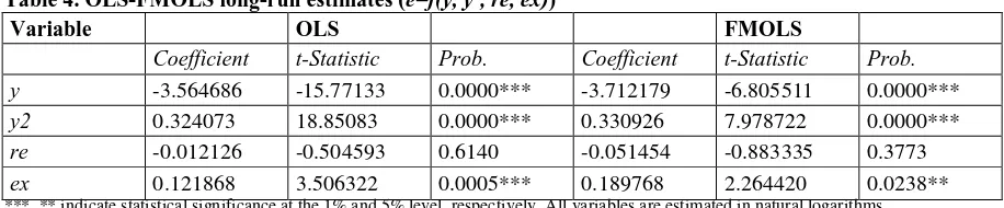
[image:10.595.69.527.132.227.2]long-run estimates for the model with exports and the model with imports are reported in Table 4 and 5, respectively. All estimated coefficients can be interpreted as long-run elasticities.
Table 4. OLS-FMOLS long-run estimates (e=f(y, y2, re, ex))
Variable OLS FMOLS
Coefficient t-Statistic Prob. Coefficient t-Statistic Prob. y -3.564686 -15.77133 0.0000*** -3.712179 -6.805511 0.0000***
y2 0.324073 18.85083 0.0000*** 0.330926 7.978722 0.0000***
re -0.012126 -0.504593 0.6140 -0.051454 -0.883335 0.3773
ex 0.121868 3.506322 0.0005*** 0.189768 2.264420 0.0238**
***, ** indicate statistical significance at the 1% and 5% level, respectively. All variables are estimated in natural logarithms.
The results of long-run estimates for the model with exports are reported in table 4. The long-run coefficients estimated from OLS and FMOLS techniques are approximately similar and have the same magnitude and produce the same sign. The validity of EKC has not been supported for the model with exports. All estimated coefficients are statistically significant except for renewable energy consumption.
[image:10.595.71.527.466.554.2]The OLS estimates results suggest that a 1% increase in per capita real GDP decrease per capita CO2 emissions by 3.56%; a 1% increase in per capita square of real GDP increase per capita CO2 emissions by 0.32%; a 1% increase in per capita real exports increase per capita CO2 emissions by 012%. The FMOLS estimates results show that a 1% increase in per capita real GDP decrease per capita CO2 emissions by 3.71%; a 1% increase in per capita square of real GDP increase per capita CO2 emissions by 0.33%; a 1% increase in per capita real exports increase per capita CO2 emissions by 0.19%. The coefficient of par capita renewable energy consumption is negative but statistically not significant under OLS and FMOLS.
Table 5. OLS-FMOLS long-run estimates (e=f(y, y2, re, im))
Variable OLS FMOLS
Coefficient t-Statistic Prob. Coefficient t-Statistic Prob.
y -3.060653 -15.93795 0.0000*** -3.094065 -6.816313 0.0000***
y2 0.302401 20.88102 0.0000*** 0.304892 8.909722 0.0000***
re 0.063592 3.562279 0.0004*** 0.058531 1.380456 0.1679
im -0.136215 -4.608848 0.0000*** -0.136413 -1.955058 0.0510*
***, * indicate statistical significance at the 1% and 10% level, respectively. All variables are estimated in natural logarithms.
For the model with imports, the long-run estimated are presented in Table 5 using OLS and FMOLS. The estimated coefficients are similar and have the same magnitude and produce similar sign. The validity of the EKC has not been supported for the model with imports. The long-run elasticities are statistically significant except for renewable energy consumption with FMOLS approach.
10 4.4. Granger causality tests
The short-run and long-run causality tests is established using Engle and Granger (1987)’s two steps. The presence of long-run relationship between emissions, real GDP, square of real GDP, renewable energy consumption, and trade openness is confirmed by Pedroni’s cointegration tests which allows for the direction of causality between variables. The approach of Engle and Granger (1987) can be used to estimate the vector error correction model.
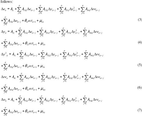
The estimation of the dynamic vector error correction model (VECM) is given as follows:
2
1 11 12 13 14
1 1 1 1
15 1 1 1
1
p p p p
it i ij it j ij it j ij it j ij it j
j j j j
p
ij it j i it it j
e e y y re
o ect
λ λ λ λ λ
λ θ µ
− − − − = = = = − − = ∆ = + ∆ + ∆ + ∆ + ∆ + ∆ + +
∑
∑
∑
∑
∑
(3)2
2 21 22 23 24
1 1 1 1
25 2 1 2
1
p p p p
it i ij it j ij it j ij it j ij it j
j j j j
p
ij it j i it it j
y e y y re
o ect
λ λ λ λ λ
λ θ µ
− − − − = = = = − − = ∆ = + ∆ + ∆ + ∆ + ∆ + ∆ + +
∑
∑
∑
∑
∑
(4)2 2
3 31 32 33 34
1 1 1 1
35 3 1 3
1
p p p p
it i ij it j ij it j ij it j ij it j
j j j j
p
ij it j i it it j
y e y y re
o ect
λ λ λ λ λ
λ θ µ
− − − − = = = = − − = ∆ = + ∆ + ∆ + ∆ + ∆ + ∆ + +
∑
∑
∑
∑
∑
(5)2
4 41 42 43 44
1 1 1 1
45 4 1 4
1
p p p p
it i ij it j ij it j ij it j ij it j
j j j j
p
ij it j i it it j
re e y y re
o ect
λ λ λ λ λ
λ θ µ
− − − − = = = = − − = ∆ = + ∆ + ∆ + ∆ + ∆ + ∆ + +
∑
∑
∑
∑
∑
(6)2
5 51 52 53 54
1 1 1 1
55 5 1 5
1
p p p p
it i ij it j ij it j ij it j ij it j
j j j j
p
ij it j i it it j
o e y y re
o ect
λ λ λ λ λ
λ θ µ
− − − − = = = = − − = ∆ = + ∆ + ∆ + ∆ + ∆ + ∆ + +
∑
∑
∑
∑
∑
(7)where ∆ is the first difference operator; the autoregression lag length, p, is set at 2 and determined automatically by the Schwarz Information Criterion (SIC); µ is a random error term; ect is the error correction term derived from the long-run relationship of Eq. (1). In order to investigate the causality relationship between emissions, economic growth, renewable energy consumption and international trade, we follow the two steps of Engle and Granger (1987). The first step consists to estimate the long-run parameters in Eq. (1) in order to get the residuals corresponding to the deviation from equilibrium. Second, we estimate the parameters related to the short-run adjustment of Eqs. (3)-(7). Short-run causality is determined by the significance of F-statistics and the long-run causality corresponding to the error correction term is determined by the significance of t-statistics. The pairwise causality is examined through the direct and indirect channels between variables.
[image:11.595.69.523.183.552.2]11
[image:12.595.75.525.216.400.2]square of real GDP) and bidirectional causality between emissions and real exports. There is also unidirectional causality running from real exports to renewable energy consumption. However, no causal links between emissions and renewable energy consumption or between economic growth and renewable energy consumption in the short-run. In the long-run, the error correction term is statistically significant for Eq. (3)-(6) and (7). However, there is a long-run relationship from i) real GDP, square of real GDP, renewable energy consumption and real exports to emissions, ii) from emissions, real GDP, square of real GDP and real exports to renewable energy consumption, and from iii) emissions, real GDP, square of real GDP, renewable energy consumption to real exports.
Table 6. Granger causality tests (model with exports) Dependent
variable Short-run Long-run
e y y2 re ex ECT
e - 4.56294 5.37836 0.06343 3.40890 -0.028628
(0.0107)** (0.0048)*** (0.9385) (0.0336)** [-2.49022]**
y 3.21787 - 0.55896 0.60753 0.00540 -0.024751
(0.0406)** (0.5720) (0.5450) (0.9946) [-0.46681]
y2 4.07499 0.57375 - 0.48470 0.02219 0.020874
(0.0174)*** (0.5637) (0.6161) (0.9781) [0.40998]
re 0.52798 1.74204 1.99969 - 4.27028 -0.057214
(0.5900) (0.1759) (0.1361) (0.0143)** [-4.38546]***
ex 3.41348 1.13377 1.20670 0.01172 -0.043958
(0.0334)** (0.3224) (0.2998) (0.9884) - [-2.30346]**
***, ** indicates statistical significance at the 1% and 10% levels, respectively. P-value listed in parentheses.
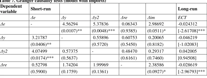
[image:12.595.73.513.609.776.2]Table 7 reports the short and the long-run relationship between emissions, economic growth, renewable energy consumption and real imports. The pairwise Granger causality results show that there is bidirectional causality between emissions and economic growth; unidirectional causality running from real imports to emissions without feedback; and unidirectional causality from real imports to renewable energy consumption in the short-run. However, there is no evidence of short-run causality links between renewable energy consumption and emissions or between renewable energy consumption and economic growth. In the long-run, the error correction term is statistically significant for Eq. (3)-(6) and (7). However, there is a long-run relationship from i) real GDP, square of real GDP, renewable energy consumption and real imports to emissions, ii) from emissions, real GDP, square of real GDP and real imports to renewable energy consumption, and from iii) emissions, real GDP, square of real GDP, renewable energy consumption to real imports.
Table 7. Granger causality tests (model with imports) Dependent
variable Short-run Long-run
e y y2 re im ECT
e - 4.56294 5.37836 0.06343 2.98692 -0.024312 (0.0107)** (0.0048)*** (0.9385) (0.0511)* [-2.61708]***
y 3.21787 - 0.55896 0.60753 0.20065 -0.046219 (0.0406)** (0.5720) (0.5450) (0.8182) [-1.02083]
y2 4.07499 0.57375 - 0.48470 0.29317 0.042005 (0.0174)*** (0.5637) (0.6161) (0.7460) [0.94508]
12
im 2.10929 0.85919 0.95274 0.02343 -0.056258
(0.1221) (0.4239) (0.3862) (0.9768) - [-3.34636]***
[image:13.595.71.514.69.101.2]***, **, * indicates statistical significance at the 1%, 5% and 10% levels, respectively. P-value listed in parentheses.
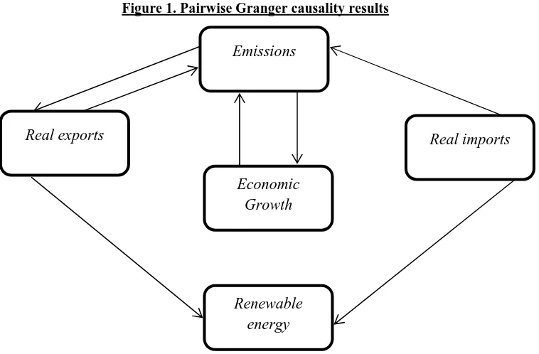
Figure 1 sums up the direct and the indirect short-run interaction between emissions, economic growth, renewable energy consumption, real exports and real imports. The interdependence between environmental indicator (CO2) and economic growth is bidirectional because real GDP (square of real GDP) Granger causes emissions and emissions Granger causes real GDP (square of real GDP). This result means that any variations in the development of economic activities will affect the emissions rate in Sub-Saharan regions and increase in the degree of pollution leads to a variation of the development of their economies. It seems that this result is not obvious given that most previous studies have not proven the bidirectional causality between economic growth and CO2 emissions. This finding is similar to Apergis et al. (2010) for a panel of 19 countries, and Halicioglu (2009) for Turkey, but not similar to the result found in Haggar (2012) for a panel of Canadian industrial sectors and Ozcan (2013) for a panel of Middle East countries and Ozturk and Acaravci (2010) for Turkey.
Figure 1. Pairwise Granger causality results
The interdependence between emissions and real exports is also bidirectional at the 5% significance level, in the short and the long-run relationship. This finding supports the feedback hypothesis. The evidence of bidirectional feedback causality between emissions and exports further implies that an increase in the CO2 emissions leads to increase the exports of merchandises. This result point out the speed and the development of merchandise exports for increasing emissions in the regions.
The direct short-run relationship between emissions and real imports is unidirectional without feedback at the 10% significance level. Thus, merchandise imports will have a positive or negative impact on CO2 emissions but, because of lack of causality, the contribution of emissions on real imports is neutral. Besides, we found evidence of a unidirectional short-run causality without feedback from trade (exports and imports) to renewable energy consumption. This causality is direct and runs from real exports to
Renewable energy
Real exports Real imports
[image:13.595.118.497.334.583.2]13
renewable energy consumption and from real imports to renewable energy consumption. This result indicates that any short-term change may affect the use of renewable energy but any increase in the share of renewable may not move the fluctuation of trade activities. This finding is not online with Ben Aïssa et al. (2014) in which they found no causality from renewable energy to trade or from trade to renewable energy either in the short or long-run. In contrast, we found an interesting result in the case of renewable energy and emissions. There is no direct causality in either direction between renewable energy consumption and emissions but there is an indirect unidirectional causality from emissions to renewable energy that runs through trade, precisely real exports. This evidence of short-run causality is explained by the fact that emissions Granger cause real exports and real exports Granger cause renewable energy consumption. This finding means that any fluctuations in the degree of carbon emissions will affect the exports of merchandise and subsequently will affect renewable energy consumption.
Also Granger short-run causality reveals no direct causality in either direction between economic growth and trade openness which means that trade openness does not derive economic growth in the region and the development economics level does not proceed to international trade. Only an indirect causality between economic growth and trade, that occurs through emissions3.
5. Conclusion and Policy Implications
We use panel cointegration techniques to investigate the long-run relationship between CO2 emissions, economic growth, renewable energy consumption and international trade for a panel of 24 Sub-Saharan countries over the period 1980-2010. Our model is based on the EKC hypothesis and follows the same methodology of Ang (2007), Halicioglu (2009) and Jayanthakumaran et al. (2012) for time series, and Haggar (2012) and Narayan and Narayan (2010) for heterogeneous panel.
To examine the causality relationship between analysis variables we develop two specification models when the dependent variable is CO2 emissions. The first model incorporates real exports and the second incorporates real imports. The aim of this separation is to specify which one of these trade variables (exports or imports) may affect environmental control (CO2) when renewable energy is used for production.
Granger causality tests reveal that, in the short-run, there is evidence of bidirectional causality between emissions and economic growth and bidirectional causality between emissions and real exports and unidirectional causality running from real imports to emissions. Also, there is no direct causality between emissions and renewable energy consumption and between economic growth and renewable energy consumption and between international trade and economic growth in the short-run. There is an indirect causality between emissions and renewable energy consumption detected through real exports. An indirect causality occurs between international trade (exports and imports) and economic growth that runs through emissions.
In the long-run, the estimates coefficients reveal that the validity of the EKC hypothesis is not established. An increase in real GDP decrease CO2 emissions, while an increase in the square of real GDP increase CO2 emissions. The estimated coefficient of renewable energy consumption is negative but statistically not significant for the model with exports. It means that any fluctuation in the use of renewable energy may not affect the degradation of the environmental indicator (CO2). In imports model, the OLS estimated coefficient of renewable energy consumption is positive and statistically significant at the 1% level, meaning that the increase in per capita renewable energy increases per capita emission.
3
14
Turning to the effect of trade openness on emissions, the impact of real exports is positive and statistically significant in both OLS and FMOLS long-run estimates. This results means that any increase in exports operations will raises emissions rate in Sub-Saharan region. The impact of real imports is negative and statistically significant in both OLS and FMOLS long-run estimates. It means that more imports operations will reduce the emissions rate.
Our policy recommendations are summarized on the fact that the authorities and policy makers of the sub-Saharan area must stimulate industrial sectors to adopt new investment strategies in renewable sources by requiring a tax policy to weak damage on the environment. Thus, the share of renewable energy sources should be increased and supported in these countries. In addition, since trade openness increases carbon emissions, the green technology investments should be supported. To do this, appropriate incentive policies should be designed by national authorities to support private sector investments on export related production and renewable energy investments. Another policy recommendation is that Sub-Saharan countries should expand their trade exchanges particularly with developed countries and try to maximize their benefit from technology transfer generated by such trade relations as this increases their renewable energy consumption.
References
Acaravci, I., Ozturk, I. 2010. On the relationship between energy consumption, CO2 emissions and economic growth in Europe”, Energy, 35, 5412-5420.
Ang, J. B., 2007. CO2 emissions, energy consumption, and output in France. Energy Policy, 35, 4772-4778.
Apergis, N., Payne, J.E., 2010a. Renewable energy consumption and economic growth evidence from a panel of OECD countries. Energy Policy, 38, 656-660.
Apergis, N., Payne, J.E., 2010b. Renewable energy consumption and growth in Eurasia. Energy Economics, 32, 1392-1397.
Apergis, N., Payne, J.E., 2011. The renewable energy consumption-growth nexus in Central America. Applied Energy, 88, 343-347.
Apergis, N., Payne, J.E., 2012. Renewable and non-renewable energy consumption-growth nexus: Evidence from a panel error correction model. Energy Economics, 34, 733-738.
Apergis, N., Payne, J.E., Menyah, K., Wolde-Rufael, Y., 2010. On the causal dynamics between emissions, nuclear energy, renewable energy, and economic growth. Ecological Economics, 69, 2255-2260.
Arouri, M.E.H., Ben Youssef , A., M′henni, H., Rault, C., 2012. Energy consumption, economic growth and CO2 emissions in Middle East and North African countries. Energy Policy, 45, 342–349.
Bekker, B., Eberhard, A., Gaunt, T., Marquard, A., 2008. South Africa's rapid electrifica-tion programme: policy, institutional, planning, financing and technical innovations. EnergyPolicy, 36, 3125–3137.
Ben Aïssa, M.S., Ben Jebli, M., Ben Youssef, S., 2014. Output, renewable energy consumption and trade in Africa. Energy Policy, 66, 11-18.
Breitung, J., 2000. The Local Power of Some Unit Root Tests for Panel Data, in: B.Baltagi (Ed.) NonStationary Panels, Panel Cointegration, and Dynamic Panels, Advances in Econometrics, 15, 161-178, JAI Press, Amsterdam.
Demirbas, M. F., Balat, M., Balat, H., 2009. Potential contribution of biomass to the sustainable energy development. Energy Conversion and Management, 50, 1746–60. Dickey, D.A., Fuller, W.A., 1979. Distribution of the estimators for autoregressive time series
15
Energy Information Administration, 2013. International Energy Outlook. EIA, Washington, DC, Available from: 〈www.eia.gov/forecasts/aeo〉.
Engle, R.F., Granger C.W.J., 1987. Co-integration and error correction: Representation, estimation, and testing. Econometrica, 55, 251-276.
Global Energy Network Institute, 2013. Available from: http://www.geni.org/ globalenergy/library/renewable-energy-resources/world/africa/wind-
africa/index.shtml.
Grossman, G., Krueger, A., 1995. Economic growth and the environment. The Quarterly Journal of Economics, 110, 353-377.
Haggar, M.H., 2012. Greenhouse gas emissions, energy consumption and economic growth: A panel cointegration analysis from Canadian industrial sector perspective. Energy Economics, 34, 358-364.
Halicioglu, F., 2009. An econometric study of CO2 emissions, energy consumption, income and foreign trade in Turkey. Energy Policy, 37, 1156-1164.
Heston, A., Summers, R., Aten, B., 2012. Penn world table version 7.1. Center of comparisons of production, income and prices at the University of Pennsylvania. Accessed at: https://pwt.sas.upenn.edu/php_site/pwt71/pwt71_form.php.
Im, K.S., Pesaran, M.H., Shin, Y., 2003. Testing for unit roots in heterogeneous panels. Journal of Econometrics, 115, 53-74.
Jalil, A., Mahmud, S.F., 2009. Environment Kuznets curve for CO2 emissions: A cointegration analysis for China. Energy Policy, 37, 5167-5172.
Jaunky, V.C, 2011. The CO2 emissions-income nexus: Evidence from rich countries. Energy Policy, 39, 1228-1240.
Jayanthakumaran, K., Verma, R., Liu, Y., 2012. CO2 emissions, energy consumption, trade and income: A comparative analysis of China and India. Energy Policy, 42, 450-460. Kaygusuz K., 2011. Energy services and energy poverty for sustainable rural development.
Renewable and Sustainable Energy Reviews, 15, 936–47.
Levin, A., Lin, C.F., Chu, C.S., 2002. Unit root tests in panel data: Asymptotic and finite- sample properties. Journal of Econometrics, 108, 1-24.
Menegaki, A. N., 2011. Growth and renewable energy in Europe: a random effect model with evidence for neutrality hypothesis. Energy Economics, 33, 257–63.
Narayan, P.K., Narayan, S., 2010. Carbon dioxide and economic growth: panel data evidence from developing countries. Energy Policy, 38, 661–666.
Ocal, O., Aslan, A., 2013. Renewable energy consumption-economic growth nexus in Turkey. Renewable and Sustainable Energy Reviews, 28, 494-499.
Ozcan, B. 2013. The nexus between carbon emissions, energy consumption and economic growth in Middle East countries: A panel data analysis. Energy Policy, 62, 1138-1147.
Ozturk, I., Acaravci, A. 2010. CO2 emissions, energy consumption and economic growth in Turkey. Renewable and Sustainable Energy Reviews, 14, 3220-3225.
Ozturk, I., Uddin, G.S. (2012), Causality among Carbon Emissions, Energy Consumption and Growth in India. Economic Research, 25(3), 752-775.
Pedroni, P., 1999. Critical values for cointegration tests in heterogeneous panels with multiple regressors. Oxford Bulletin of Economics and Statistics, 61, 653-678.
Pedroni, P., 2001. Purchasing power parity tests in cointegrated panels. The Review of Economics and Statistics, 83, 727-731.
16
Sadorsky, P., 2009a. Renewable energy consumption, CO2 emissions and oil prices in the G7 countries. Energy Economics, 31, 456-462.
Sadorsky, P., 2009. Renewable energy consumption and income in emerging economies. Energy policy, 37, 4021-4028.
Sadorsky, P., 2012. Energy consumption, output and trade in South America. Energy Economics 34, 476-488.
Shahbaz, M., Lean, H.H., Shabbir, M.S., 2012. Environmental Kuznets Curve hypothesis in Pakistan: Cointegration and Granger causality. Renewable and Sustainable Energy Reviews, 16, 2947-2953.
Suberu, M. Y., Mustafa, M. W., Bashir, N.,Muhamad, N. A., Mokhtar, A. S., 2013. Power sector renewable energy integration for expanding access to electricity in sub-Saharan Africa. Renewable and Sustainable Energy Reviews, 25, 630-642.
Phillips, P.C.B., Perron, P., 1988. Testing for a unit root in time series regressions. Biometrika, 75, 335-346.
United Nations Environment Programme, 2012. Financing renewable energy in developing countries. Geneva, Switzerland.
Yildirim, E., Sarac S., Aslan., A., 2012. Energy consumption and economic growth in the USA: Evidence from renewable energy. Renewable and Sustainable energy Reviews, 16, 6770-6774.