Dynamic Stall on Vertical Axis Wind Turbines

(1)

Dynamic Stall on Vertical Axis Wind Turbine Blades

Thesis by

Reeve Dunne

In Partial Fulfillment of the Requirements

for the Degree of

Doctor of Philosophy

California Institute of Technology

Pasadena, California

2016

(2)

c 2016

Reeve Dunne

(3)

Acknowledgments

I would like to first thank my advisor Beverley McKeon for working with and advising me over the past five years. It has been an honor to have spent this time in her group, and I have learned a great deal with her support. Furthermore I’d like to thank the rest of my committee: Tim Colonius, John Dabiri, and Melany Hunt, for reviewing this thesis and providing their insight on my work.

I would also like to thank Morteza Gharib and David Jeon for sharing and providing support for the facility used for this research, as well as Peter Schmid, without whose insight and experience with the dynamic mode decomposition much of this work would not have been possible. While performing this work, I have had the opportunity to collaborate with Hsieh-Chen Tsai, who provided another view of the challenges in this thesis. Additionally I benefited from discussions on vertical axis wind turbines with Daniel Araya, Matthias Kinzel, Julia Coss´e and others.

It has been a privilege to work with the students and faculty of both mechanical engineering and GALCIT. I especially want to thank my first year advisor, Guillaume Blanquart, as well as my colleagues in the McKeon group, and everyone who started with me in 2010, notably Esteban Hufstedler for the many conversations we’ve had that have made their way into this thesis.

To my friends from Caltech to Tufts and from California to Colorado and Massachusetts, I can not thank you enough for your friendship and for listening to stories from my research. All the time I have spent at Caltech in the classroom, laboratory, or on the softball field, or outside biking, hiking, skiing, or sailing, you have made all these years unforgettable. Thank you to Kathleen Keough for her support for this thesis and beyond.

Finally thank you to my family: my mother Diane Dunne, Aunt and Uncle, Monk and Bob Ward. Without your tireless love and support none of this would have been possible.

(4)

Abstract

In this study the dynamics of flow over the blades of vertical axis wind turbines was investigated using a simplified periodic motion to uncover the fundamental flow physics and provide insight into the design of more efficient turbines. Time-resolved, two-dimensional velocity measurements were made with particle image velocimetry on a wing undergoing pitching and surging motion to mimic the flow on a turbine blade in a non-rotating frame. Dynamic stall prior to maximum angle of attack and a leading edge vortex development were identified in the phase-averaged flow field and captured by a simple model with five modes, including the first two harmonics of the pitch/surge frequency identified using the dynamic mode decomposition. Analysis of these modes identified vortical struc-tures corresponding to both frequencies that led the separation and reattachment processes, while their phase relationship determined the evolution of the flow.

Detailed analysis of the leading edge vortex found multiple regimes of vortex development coupled to the time-varying flow field on the airfoil. The vortex was shown to grow on the airfoil for four convection times, before shedding and causing dynamic stall in agreement with ‘optimal’ vortex formation theory. Vortex shedding from the trailing edge was identified from instantaneous velocity fields prior to separation. This shedding was found to be in agreement with classical Strouhal frequency scaling and was removed by phase averaging, which indicates that it is not exactly coupled to the phase of the airfoil motion.

(5)

List of Figures

1.1 Periodic velocity and Reynolds number variation over typical VAWT blade, forη= 2,

U∞= 5m s−1, c= 15cm (solid lines). Compared to test motion (dashed lines). . . 3

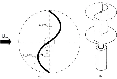
1.2 Top view schematic of typical drag based VAWT (left). Clockwise rotation is driven by

drag coefficient discrepancy between advancing and receding blades. (Right) Isometric

view of drag based Savonius turbine from Hau (2013). . . 5

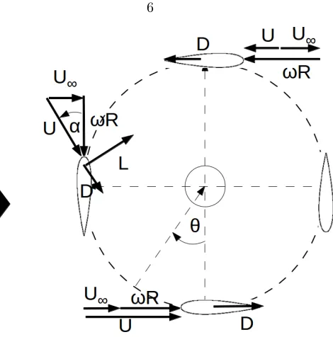
1.3 Top view of a typical VAWT. Wind speedU∞, relative velocityU, blade velocityωR,

lift L and drag D, directions. Clockwise rotation is driven by lift on each blade. θ

denotes angular location with zero corresponding to maximum relativeU andα= 0◦. 6

2.1 Tunnel schematic (Lehew, 2012) . . . 15

2.2 CAD model of the pitch/surge mechanism. . . 16

2.3 Picture of pitch/surge apparatus installed in test section. . . 17

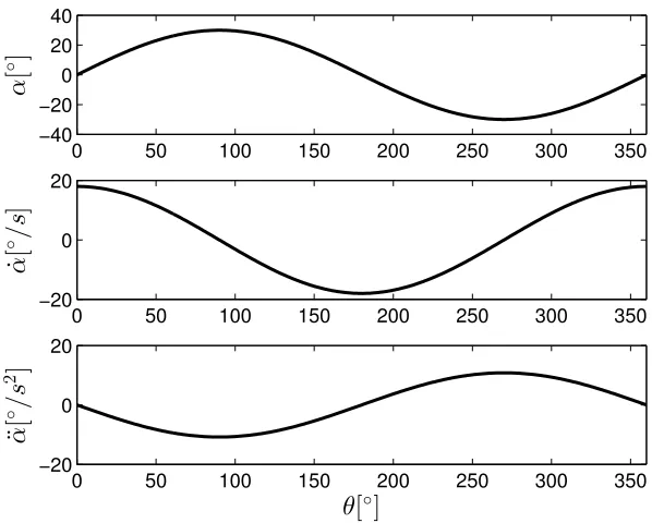
2.4 Angle of attackα, dα dt, and

d2α

dt2.. . . 18

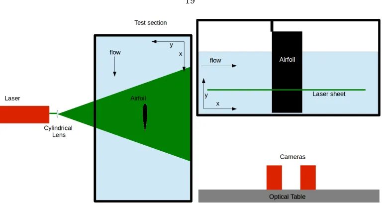
2.5 Schematic of PIV setup for streamwise/cross-stream measurements. . . 19

2.6 Schematic of PIV setup for streamwise/spanwise measurements. . . 20

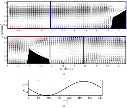
2.7 (a. top) Experimental field of view in laboratory frame. Front and back fields of view

shown in red and blue, respectively. Top panel shows airfoil in maximum aft position,

bottom in maximum forward position for pitch/surge and surging motion (pitch/surge

shown). Pitch only experiments were performed only in the front field of view, at the

maximum forward positionxl= 1 shown in the top panel. (b. bottom) Plot of leading

edge positionxl in airfoil motion cycle. . . 22 2.8 Field of view in the airfoil-fixed frame. Time is extruded in the z direction to show

entire time series in one image. White lines show how field of view moves around in

(9)

2.9 Top view of a VAWT demonstrating experimental field of view in rotating VAWT

frame. Wind speedU∞, effective velocity U, blade velocity ωR. Experimental field of

view shown by grey boxes (not to scale).. . . 24

2.10 Mean streamwise velocityuforα= 10◦(a),α= 15◦ (b) andα= 20◦ (c) scaled by the freestream velocity ¯U, atz= 200mm (x/y measurement domain). . . 29

2.11 Contour plots of averageuvelocity, scaled by the freestream velocity ¯U, measured in

x/zplane at static angles of attack. Airfoil leading edge atx= 0. Water tunnel floor at

z= 0 (units in mm), water depth 457mm. x/ymeasurement plane/laser atz∼200mm

shown by green line on plots. . . 30

2.12 Mean spanwise velocity w scaled by the freestream velocity ¯U, at z = 200mm (x/y

measurement domain).. . . 32

2.13 Contour plots of average w velocity, scaled by the freestream velocity ¯U, measured

in x/z plane at static angles of attack. Airfoil leading edge at x= 0. Water tunnel

floor atz = 0 (units in mm), water depth 457mm. x/y measurement plane/laser at

z∼200mm shown by green line on plots. . . 33

2.14 Variance ofuandwatz= 200mm (x/y measurement domain)α= 15◦. . . 34

2.15 Vector plot instantaneous vector field for airfoil atα= 15◦. . . 34

2.16 Contour plots of averageuvelocity, scaled by the freestream velocity ¯U, measured in

x/z plane at static angles of attack onc = 100mm AR= 4.6 airfoil atRe = 50,000.

Airfoil leading edge atx= 0. Water tunnel floor atz= 0 (units in mm), water depth

457mm. x/y measurement plane/laser atz∼200mm shown by green line on plots.. . 36

2.17 Contour plots of averagewvelocity, scaled by the freestream velocity ¯U, measured in

x/z plane at static angles of attack onc = 100mm AR= 4.6 airfoil atRe = 50,000.

Airfoil leading edge atx= 0. Water tunnel floor atz= 0 (units in mm), water depth

457mm. x/y measurement plane/laser atz∼200mm shown by green line on plots.. . 37

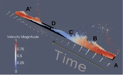
3.1 Vorticity isocontour colored by scaled velocity magnitude (

√

u2₊_v2

max(√u2+v2)). 1.2 periods

shown. Arrows indicate incoming angle of attack variation. Points A, A’ correspond to

α+ = 0, B to separation location, C to reattachment, D to minimum angle of attack.

Note that at point D flow at and behind the trailing edge cannot be measured. The

location of points A-A’ on pitch/surge period showin in figure 3.2 . . . 40

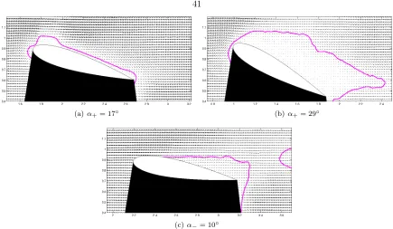
3.2 Location of points A-A’ from figure 3.1 in pitch/surge cycle. Angle of attack α(top)

(10)

xvelocity u= 0.25U in magenta. (a) Pitch up before separation, (b) near maximum

angle of attack after separation, and (c) on pitch down nearing reattachment. . . 41

3.4 Expanded view of the vorticity isocontour from figure 3.1 leading up to separation.

Clockwise vorticity in blue, counter-clockwise in red. The emergence of a trailing

edge vortex is apparent at pointβ. Point B indicates separation location just before

maximum angle of attack (denoted by the green sheet). . . 42

3.5 Expanded view of the leading edge vorticity isocontour from figure 3.1 during pitch

up, with the maximum angle of attack indicated by the green sheet. The vorticity

isocontour retreats around the airfoil leading edge until separation at point B. Vorticity

isocontour, colored by scaled velocity magnitude, as in figure 3.1.. . . 43

3.6 Velocity (vectors) and vorticity (contour), scaled by maximum modal vorticity, plots

of time constant λi = 0 mode in airfoil-centered frame from a single DMD mode.

Incoming flow and the diffuse vorticity associated with flow curvature around the airfoil

are captured. . . 43

3.7 Modes calculated with DMD scaled by pitch surge frequency Ω. λr growth rate λi

frequency. Point size scaled by the magnitude of the spatial structure, a. Left full

spectrum, right zoomed in on strong, non-decaying modes. Modes circled in green

used for further analysis. . . 44

3.8 Isocontour of vorticity (colored by scaled velocity magnitude) of data (left) and

five-mode DMD reconstruction (right) for entire data set. Reconstruction captures primary

behavior of flow. . . 45

3.9 Normalized circulation within leading edge vortex of five-mode DMD model (+) and

data (o). Plotted against airfoil angle of attack,α. . . 46

3.10 Location of plots a-e on pitch surge cycle for first (a) and second (b) mode pairs in

figures 3.11 and 3.12, respectively. . . 48

3.11 Velocity and vorticity (scaled by maximum modal vorticity) plots of first DMD

conju-gate pair at pitch/surge frequency Ω with the freestream velocity variation from surge

removed. Vortex structure at leading edge apparent in figures a and e. Maximum

(11)

3.12 Velocity and vorticity (scaled by maximum modal vorticity) plots of second DMD

conju-gate pair at twice pitch/surge frequency 2Ω. Maximum velocity magnitude (√u2₊_v2₎

30% of freestream velocity ¯U. . . 50

3.13 Schematics of the primary (a) and secondary (b) separation modes at first and second

harmonic of pitch/surge frequency Ω. Vortex in the primary mode leads separation

and lags reattachment, vortex in secondary mode lags separation convecting along the

shear layer, and leads reattachment. . . 51

3.14 Primary (blue) and secondary (green) separation mode strengths over 2 airfoil cycles.

Lines at separation and reattachment points B and C. Modes interact constructively

on the suction side of airfoil (0 ≤ α ≤ 30) and destructively on the pressure side

(0≥α≥ −30). . . 51

4.1 Leading edge vortex circulation, diameter, and position over half a pitch up/down cycle

α≥0. . . 56

4.2 Location of points A-A’ from figure 3.1 in pitch/surge cycle. Angle of attack α(top)

Reynolds number (bottom). . . 56

4.3 Γ2= 2.2/πcontour of identified leading edge vortex colored by vorticity. Positive angle

of attack half of pitch/surge period shown. Time shown from right to left to provide

best angle to view vortex structure. . . 57

4.4 Vorticity contour with velocity vector plot near the beginning of LEV formation (α=

19◦). Γ2= 2/πcontour in white at the leading edge of the airfoil. . . 58

4.5 Isocontour of Γ2 = 2.2/π colored by vorticity seen from below indicating the leading

edge vortex during the development regime beginning at point Φ, at the left side of

the isocontour and ending at B on the right side of the contour. From this angle the

primary core of the vortex can be seen as a circular structure. This structure remains

just above the leading edge of the airfoil, which has been removed from the image, so

the shape of the vorticity isocontour can be observed. . . 58

4.6 Vorticity contours from phase-averaged realization (left) and instantaneous (right) from

the front field of view. Red and blue contours indicate positive and negative vorticity,

respectively. The green area indicates the PIV laser shadow. . . 60

(12)

aft field of view forα= 9◦(top) and 19◦(bottom). Some vorticity can be seen behind the trailing edge, but no coherent periodic shedding is observed. . . 62

4.9 Vorticity contour plots, with velocity vector fields at the same contour level as figure

4.8 from the instantaneous data set in the aft field of view forα= 9◦ (top) and 19◦ (bottom). Shed vortices clear behind trailing edge. . . 63

4.10 DMD mode spectrum performed on the instantaneous data set in the aft field of view.

λrandλimodal growth rate and frequency, respectively. Point size determined by the

relative spatial amplitude of the mode.. . . 64

4.11 Vorticity contour plot of the DMD modes betweenF = 3 and 12 Hz at α= 19◦. . . . 65

4.12 Vorticity contour plots of the DMD modes forF = 5−8 Hz (a) andF = 8−12 Hz (b)

atα= 19◦using the same contour level as figure 4.11. . . 65

4.13 Vorticity contour plot of the DMD modes betweenF = 3 and 12 Hz at α= 9◦. . . 66

4.14 Vorticity contour plot of the DMD modes between F = 5 and 8 Hz atα= 9◦ at the same contour level as figure 4.13. . . 66

4.15 Vorticity contour plots of DMD modes betweenF = 5−6 Hz. α= 9◦ (top), α= 19◦ (bottom). . . 67

4.18 Vorticity isocontour of DMD modes with frequencies between 1.5 ≤F ≤10 Hz over

the pitch up cycle 0◦≤α+≤30◦. . . 69

4.19 Schematic of the time extrusion for 0◦ ≤ α± ≤ 30◦ demonstrating the regions in

which each timescale effects the flow. A corresponds toα+= 0◦and C corresponds to

α− = 0◦. White lines correspond to each location A, B, C, Φ, and Ψ in extruded time. 70

4.20 Time extrusion for 0◦≤α±≤30◦. The top figure shows the phase averaged spanwise

vorticity (colored by velocity magnitude), and trailing edge vortex shedding determined

from DMD in the range 1.5≤F <9.5 Hz (alternating red and blue contours behind

the airfoil), Finally in the bottom the Γ2 = 2.2/π contour shows LEV development

in relation to the trailing edge shedding. The trailing edge vortex shedding has been

(13)

5.1 Vorticity isocontour for sinusoidal pitch (bottom) and combined pitch/surge motion

(top) colored by velocity magnitude. Two periods shown beginning at Aθ= 0◦, α= 0◦ maximum surge velocity as in figure 1.1. Arrows indicate incoming angle of attack

variation. Φ indicates the beginning of leading edge vortex growth, B at separation

location, C at the beginning of reattachment. . . 76

5.2 Leading edge vortexxposition (top) and circulation (bottom) over half a pitch up/down

cycleα≥0 for pitch (blue) and combined (red) cases. . . 77

5.3 Γ2= 2.2/πisocontour of identified leading edge vortex colored by vorticity magnitude

for half a pitch up/down cycle α ≥ 0 (Pitch/surge (top), pitch (bottom)). Time is

from right to left. A, Φ, B, Ψ, and C correspond to figure 5.2, based on changes in the

pitch/surge flow field. Gaps exist where Γ vortex criteria are not met. . . 78

5.4 Leading edge vortex circulation andxposition plotted against airfoil convection time

for pitch up/pitch down half periodα≥0. ˆT = 0 corresponds toθ= 0◦,α+ = 0◦. . . 80

5.5 Modes calculated with DMD for pitch-only motion scaled by pitch frequency Ω. λr

growth rateλi frequency. Point size scaled by the magnitude of the spatial structure,

a. Left full spectrum, right zoomed in on strong, non-decaying modes. Modes circled

in green used for five-mode model, red modes used for seven-mode model. . . 81

5.6 Isocontour of vorticity (colored by scaled velocity magnitude) of the five-mode DMD

reconstruction (left) and data (right) focused on point of dynamic stall. Vectors show

the incoming velocity field. Model captures separation point, but misses flow detail. . 82

5.7 Isocontour of vorticity (colored by scaled velocity magnitude) of the seven-mode DMD

reconstruction (left) and data (right) focused on point of dynamic stall. Vectors show

the incoming velocity field. Shear layer and reattachment shape captured with the

addition ofλi=±3Ω mode to the reconstruction in figure 5.6. . . 83

5.8 Isocontour of vorticity of seven-mode (top) and five-mode (bottom) DMD

reconstruc-tion (left) and data (right) zoomed in on the separated region. Unlike the five-mode

model, the seven-mode model captures the details of the separated region, including

reattachment point. . . 85

5.9 Velocity (vectors) and vorticity (contour), scaled by maximum modal vorticity, plots of

time constant base flow in airfoil-centered frame from a single DMD mode. Incoming

(14)

of first DMD conjugate pair at pitch frequency Ω. Vortex structure at leading edge

apparent in figures a and e. Maximum velocity magnitude (√u2₊_v2 _∼ _{100% of}

freestream velocity ¯U). . . 87

5.11 Velocity (vector) and vorticity (contour) (scaled by maximum modal vorticity) plots

of second DMD conjugate pair at twice the pitch frequency Ω. Maximum velocity

magnitude (√u2₊_v2_∼_{44% of freestream velocity ¯}_U_). _{. . . .} ₈₈

5.12 Velocity (vectors) and vorticity (contour), scaled by maximum modal vorticity, plots of

the secondary separation mode (λi=±2Ω and±3Ω) during pitch up and pitch down,

respectively. Maximum velocity magnitude (√u2₊_v2_∼_{27% of freestream velocity ¯}_U_). ₈₉

5.13 Time varying strengths of the mode pairs at the first three harmonics of the pitch

frequency used in figure 5.7. λi =±Ω in blue λi =±2Ω in black, andλi =±3Ω in

red. Combined second and third pair (λi =±2Ω and±3Ω) plotted in dashed lines.. . 90

5.14 Vorticity isocontour for surging motion atα= 20◦(top) andα= 15◦(bottom) colored by velocity magnitude. Two periods shown starting at maximum surge velocity as in

figure 5.1(a). . . 92

5.15 Vorticity isocontour for surge motion at α = 15◦ just after point ζ (figure 5.14(b)). Flow is seen to separate around pointas the airfoil accelerates forward. . . 93

6.1 Vorticity contours from experiment. Phase-averaged realization (left) and

instanta-neous (right) from the aft field of view. In the instantainstanta-neous realization atα+ = 19◦

the measurement is cut off over the leading edge due to the aft field of view. Red

and blue contours indicate positive and negative vorticity, respectively. The green area

indicates the PIV laser shadow.. . . 98

6.2 Vorticity contours from experiment. Phase-averaged realization (left) and

instanta-neous (right) from the front field of view. Red and blue contours indicate positive and

negative vorticity, respectively. The green area indicates the PIV laser shadow. . . 99

6.3 Vorticity contours from the computations of Tsai and Colonius (2014) at the same

angular location as the experiment in figure 6.1. Planar motion EPMC _{(left) and}

turbine frame VAWTC _{(right). Red and blue contours indicate positive and negative}

(15)

6.4 Vorticity contours from the computations of Tsai and Colonius (2014) at the same

angular location as the experiment in figure 6.2. Planar motion EPMC _{(left) and}

turbine frame VAWTC _{(right). Red and blue contours indicate positive and negative}

vorticity, respectively. . . 101

6.5 Clockwise vorticity contours from experiment (EPME_{) (top) and VAWT computation}

(VAWTC) (bottom from Tsai and Colonius (2014)) at θ = 70◦, 90◦, 108◦, and 133◦, respectively, from left to right. . . 102

6.6 Dynamic stall regimes from 4.19 in VAWT frame. Dynamic stall development (green),

trailing edge vortex shedding (magenta), leading edge vortex development (red), and

separated flow (blue). . . 105

6.7 Clockwise vorticity contours on the upstream half of a representative three-bladed

turbine turbine. . . 105

(16)

Nomenclature

t Time [s]

AR Aspect ratio

α Angle of attack [◦]

θ Turbine rotation angle [◦]

Rec Chord Reynolds number (U c_ν )

U∞ Windspeed [m s−1]

U Effective velocity/Freestream velocity relative to airfoil [m s−1_]

¯

U Average velocity in experiment (tunnel velocity) [m s−1]

χ Vorticity [s−1]

η Tip speed ratio (_UωR ∞)

ω Turbine frequency [rad s−1_]

Ω Pitch/surge frequency [rad s−1_] R Turbine radius [m]

Ro Rossby number (U∞

2cω)

c Chord length [cm]

th Airfoil thickness [m]

ν Kinematic viscosity [m2 _s−1_]

λ Transformed DMD eigenvalues [rad s−1]

k Reduced frequency [_{2 ¯}Ω_Uc] Γ1 Vortex center criterion

Γ2 Vortex boundary criterion

(17)

uΓ Vortex circulation [m2 s−1] xv Vortex x position [c] ∆α Pitch amplitude [◦]

α0 Mean angle of attack [◦]

αss Static stall angle [◦] ˆ

T Formation time/airfoil convection time ( ˆT =R U_cdt)

F Frequency [Hz]

St Strouhal number [F c_U]

subscript

i Imaginary component

r Real component

j Variable index

(18)

List of Abbreviations

VAWT Vertical axis wind turbine HAWT Horizontal axis wind turbine DMD Dynamic mode decomposition LEV Leading edge vortex

TEV Trailing edge vortex PIV Particle image velocimetry EPM Equivalent planar motion

superscript

C Computational

(19)

Chapter 1

Introduction

1.1 Motivation

In 2014 the United States produced approximately 4.1 trillion kilowatt-hours of electricity. Sixty-seven percent of this electricity was generated using fossil fuels, predominantly coal and natural gas (US Energy Information Administration, 2015). This produced approximately 2000 metric tons of greenhouse gas emissions (Environmental Protection Agency,2015). To curtail this greenhouse gas pollution and reduce the dependence on fossil fuels, more renewable energy sources are being utilized. Since 2012, wind energy has been the leading source of new generating capacity in the United States, producing 4.4% of the total production in 2014 (up from 3.6% in 2013) (American Wind Energy Association,2013; US Energy Information Administration,2015). Most of this energy is currently produced using large scale horizontal axis wind turbines (HAWTs) that can individually generate over three megawatts of electricity, with blade diameters up to 126m (Vestas, 2015). Individual HAWTs are very efficient, extracting nearly the theoretical Betz limit of 59% of the power of the wind (Vanek and Albright,2008). The power output from wind farms however is limited by interference between the turbines. Due to this interference turbines must be separated by three to five turbine rotor diameters in the cross stream direction and six to ten diameters downstream to achieve an average of 90% of individual turbine efficiency (Hau,2013). This restriction limits the power density (defined as power produced per unit of land area) to 2-3W m−2 ₍_MacKay_,₂₀₀₉_).

(20)

that larger arrays could maintain up to 18W m−2_{, even with the resulting decreased freestream}

velocity apparent to interior turbines in the larger array. Kinzel et al. (2012) measured the flow field within similar eighteen turbine arrays and demonstrated that flow velocity returned to 95% of upwind velocity within six diameters of a counter-rotating VAWT pair, significantly faster than from behind typical HAWTs. In addition to the lower spacing requirements, VAWTs have the advantages of an insensitivity to wind direction, quieter running conditions due to slower blade motion, and a typically simpler design, resulting in construction with fewer moving parts and a constant blade profile along the span (Greenblatt et al., 2013; Islam et al., 2007). While modern HAWTs can approach theoretical maximum efficiency, the aerodynamics of VAWTs are less well understood, and their individual efficiency suffers, such that even the best VAWT designs are≥10% less efficient than HAWTs (Hau,2013). Furthermore, this increased aerodynamic complexity increases the dangers of fatigue loading, decreasing the reliability of VAWTs in the field, and causing sometimes catastrophic failure (Dabiri et al., 2015; Coss´e,2014).

This work studies an approximation of the flow experienced by an individual blade of a vertical axis wind turbine as a first step to understanding the complex fluid dynamics that limits the efficacy of current VAWT designs. The variation in flow conditions caused by the rotation of the turbine is decomposed into a time dependent angle of attack and velocity variation. This variation is reproduced in the lab by pitching and surging an airfoil sinusoidally at the same chord Reynolds number, phase, and reduced frequency as a representative VAWT blade introduced in section1.2.1

in a water tunnel described in Chapter2. A comparison of the turbine kinematics given by equation

1.1to the sinusoidal pitch/surge motion used in the experiment is shown in figure1.1.

α= tan−1

_sin_θ

η+ cosθ

(1.1a)

U =U∞

p

1 + 2ηcos (θ(t)) +η2 _(1.1b)

Pitching and surging motion can capture the angle of attack and velocity variation of the turbine; however, it neglects the the Coriolis effect due to the rotation of the turbine. The Coriolis force imposes a force on the flow to account for the curved path of the turbine blade. The relative importance of this Coriolis force in a VAWT can be measured using the ratio of inertial to rotational forces, the Rossby number (Ro = U∞

(21)

0 50 100 150 200 250 300 350 −20 0 20 B la d e α

0 50 100 150 200 250 300 350 0.5

1 1.5

x 105

B la d e R ec

Turbine Angleθ

Static Stall NACA0018

Figure 1.1: Periodic velocity and Reynolds number variation over typical VAWT blade, for η = 2,

U∞= 5m s−1,c= 15cm (solid lines). Compared to test motion (dashed lines).

the turbine, Ro= ₂_∗R_c_∗_η. For a standard industrial turbine atη = 2, c= 15cm (Windspire,2013) the Rossby number is order 1. The effect of the Coriolis force, discussed further in section 1.2.1

and Chapter 6, has been studied by Tsai and Colonius (2014), who demonstrated a similar flow development prior to flow separation with and without the Coriolis force at a much lower Reynolds number.

(22)

Numerous authors have performed both experimental and computational research on the flow over airfoils, including dynamic and static stall over a wide range of conditions such as Reynolds number, Mach number, airfoil shape, etc. A review of the most applicable work to vertical axis wind turbine flows, focusing on incompressible flow, over simple airfoils is summarized below to provide context for this work.

For the rest of the thesis, streamwise, cross-stream and spanwise directions are denoted byx,y

andz, respectively, with associated velocitiesu,v, andw and spanwise vorticity

χ= ∂v

∂x −

∂u

∂y. (1.2)

1.2.1 Vertical axis wind turbines

The oldest designs of vertical axis wind turbines are driven purely by drag, similar to cup anemome-ters used to measure wind velocity. A schematic of a drag based VAWT is shown in figure1.2. These designs are based on a drag differential between the advancing (−90◦ _{< θ <} ₉₀◦_{) and retreating}

(90◦< θ <270◦) blades and are limited to a tip speed ratio defined as the blade speed divided by the incoming windspeed, η= _UωR

∞ <1, whereR is the radius of the turbine,U∞ is the free stream wind velocity, and ω the turbine rotation rate, since the blade velocity cannot exceed that of the wind pushing it. This tip speed ratio limitation decreases the turbine efficiency significantly (Hau,

2013).

(23)

[image:23.612.127.506.81.338.2]

(a) (b)

Figure 1.2: Top view schematic of typical drag based VAWT (left). Clockwise rotation is driven by drag coefficient discrepancy between advancing and receding blades. (Right) Isometric view of drag based Savonius turbine fromHau(2013).

investigated the effect of using different airfoils for small straight bladed VAWTs and concluded that due, partially to the difference in velocity in upstream and downstream halves of the turbine, thick, high lift, asymmetrical airfoils are often best suited for VAWTs. Furthermore,Beri and Yao(2011) found that using a cambered airfoil aided in the self-starting ability of the turbines, allowing the turbines to spin at a lower windspeed. A schematic of a typical lift based VAWT is shown in figure

1.3, demonstrating angle of attackα, effective velocityU, and the directions of the typical lift and drag vectors. Only these modern, lift-driven turbines are considered in this study.

Araya and Dabiri(2015) measured the wake of lift driven VAWTs over a range of tip speed ratios and Reynolds numbers. They performed experiments on turbines driven by the flow, with the tip speed ratio controlled by a brake, and/or driven by a motor. They found that the wake was affected most strongly by tip speed ratioη, while Reynolds number had a minor effect. Furthermore, they found that while the wake was changed when the tip speed ratio was driven beyond what it could achieve without a motor, if the tip speed ratio and Reynolds number were kept constant, there was no difference between a flow or motor driven turbine.

(24)

[image:24.612.218.453.54.292.2]

Figure 1.3: Top view of a typical VAWT. Wind speed U∞, relative velocityU, blade velocity ωR,

lift L and drag D, directions. Clockwise rotation is driven by lift on each blade. θ denotes angular location with zero corresponding to maximum relativeU andα= 0◦.

low tip speed ratios this angle of attack variation drives the airfoil well above its static stall angle, resulting in dynamic stall on each blade twice per turbine cycle, once on each side of the blade (figure 1.1). In practical terms dynamic stall causes an abrupt drop in the lift of the blade, and therefore torque on the turbine, as well as potentially damaging unsteady loading on the generator and turbine structure (Greenblatt et al.,2013); error in predicting these dynamic loads can decrease VAWT lifetimes by a factor of up to 70 (Carr, 1988). In addition to dynamic stall, the blade also experiences attached and separated flow during different portions of the rotation cycle. Each of these regimes exerts different forces on the turbine and must be considered in the design of an efficient and robust VAWT.

1.2.2 Dynamic stall

In addition to vertical axis wind turbines, dynamic stall appears in many aspects of unsteady aero-dynamics from helicopters to micro air vehicles. In biological and bio-inspired aeroaero-dynamics the increased lift production experienced during dynamic stall is critical in achieving flight (Rival et al.,

(25)

review of only the most pertinent literature to vertical axis wind turbines.

Dynamic stall is understood to correspond to significant differences in the flow field and forces during pitch-up and pitch-down on an airfoil undergoing unsteady motion. During pitch up, there is significant stall-delay resulting in attached flow, and high lift well beyond the static stall angleαss. Additionally, during pitch up a leading edge, or dynamic stall vortex, is expected to develop, and subsequently shed from the airfoil, with an associated drop in lift. On pitch down there is a similar delay in the flow reattachment.

In a technical report for NASA, Carr et al.(1977) performed some of the first experiments on dynamic stall on NACA 0012 and other airfoils with a pitch amplitude of ∆α∼10◦_{and mean angle}

of attack (α0 = 15◦). These experiments, performed at Reynolds numbers up to 2.5×106, used

flow visualization to identify leading edge vortex (LEV) development, growth, and shedding. After sufficient time the LEV was shown to begin to move aft until it reached the airfoil trailing edge, when it was finally shed from the airfoil and convected downstream. Combining these visualizations with force measurements, they were able to show that pitching moment about the quarter-chord decreases substantially when the vortex moves aft, and, finally, when the vortex reaches the trailing edge and sheds the lift stops increasing with increasing angle of attack. These points are defined as ‘moment stall’ and ‘lift stall’, respectively, and in this dynamic case do not occur at the same angle of attack as they do on static airfoils.

Particle image velocimetry analysis atRe= 9×105_{was performed by}_{Mulleners and Raffel}₍₂₀₁₂_, 2013) on a cambered airfoil pitching ∆α= 6−8◦ around a statically attached, but high angle of attack betweenα0= 18◦andα0= 22◦ at reduced frequencies betweenk= _{2 ¯}ωc_U = 0.05−0.10, where c is the airfoil chord, ω is the angular frequency, and ¯U is the mean velocity. These experiments highlighted five stages of the flow corresponding to attached flow, stall development, stall onset, stall, and flow reattachment (Mulleners and Raffel, 2012) and identified a ‘primary stall vortex’ pinched off at the point of dynamic stall (Mulleners and Raffel, 2013). Furthermore, a distinction was made between light and deep dynamic stall, where light stall was characterized by a much smaller separation region. Mulleners and Raffel (2012) show that deep stall was caused when the dynamic stall vortex separated before maximum angle of attack, while light stall occurred when the vortex separated from the airfoil as a result of the change of pitch direction at the maximum angle of attack.

Similar pitching experiments on a flat plate at a lower Reynolds number betweenRe= 5×103

(26)

motion period, or at a higher angle of attack, with increasedkin agreement with the results ofRival et al. (2009). They showed that leading edge vortex circulation tended to increase linearly with the phase of the airfoil motion, with a faster growth corresponding to a lower reduced frequency

k. Baik and Bernal (2012) andKang et al. (2013) performed experiments and computations on a SD7003 airfoil under similar conditions, demonstrating a phase delay of the dynamic separation on the airfoil when compared to the flat plate due to increased attachment over the smoothed leading edge. Furthermore, the unsteady lift peak was shown to be higher in the flat plate case, while the average lift was increased in the airfoil case due to the flow remaining attached up to a higher angle of attack.

Rival et al.(2009) found that a strong trailing edge vortex (TEV) appears when the LEV sheds and convects past the airfoil at the point of lift stall. The TEV was shown to cause a significant decrease in lift similar to the effects of a starting vortex. This lift deficit remained for a significant portion of the airfoil motion cycle (Rival et al., 2009; Panda and Zaman, 1994). In further work

Prangemeier et al.(2010) tested different pitch motions at the bottom of a plunge motion to mitigate the effect of the trailing edge vortex TEV. Using a ‘quick pitch’ motion, they were able to reduce the TEV circulation by at least 60%.

Choi et al. (2015) investigated surging and plunging airfoils computationally at Re = 500 and experimentally atRe= 5.7×104_{. In surging experiments they found attenuation or amplification of}

the unsteady forces, depending on the reduced frequencykof the motion. Atk= 0.7 the LEV was shed while the airfoil was advancing, increasing the already high lift due to the higher velocity, thus amplifying the unsteady force component. In the k= 1.2 case the LEV was shed while the airfoil was retreating and as such, added to the relatively low lift during retreat, decreasing force variation. In order to reduce the negative effects of dynamic stall;Heine et al.(2013) placed passive distur-bance generators near the leading edge of an airfoil pitching ∆α= 5◦ and 7◦ about α0 = 13◦ and demonstrated a significant decrease in the lift drop after dynamic stall. PIV measurements were used to show that the perturbed airfoil exhibited a smoother stall from the trailing edge forward instead of the abrupt leading edge separation exhibited in classical dynamic stall. Greenblatt and Wygnanski(2001) andGreenblatt et al.(2001) used oscillatory and steady blowing on airfoils at the leading edge, and over a trailing edge flap at high Reynolds number (Re≥3×106_{) under various}

(27)

elimi-nate the leading edge vortex, removing lift hysteresis and mitigating trailing edge separation, thus increasing overall lift.

M¨uller-Vahl et al.(2015) used PIV and pressure measurements on a NACA-0018 airfoil pitched about the quarter-chord at k= 0.074 to investigate the effect of constant blowing near the leading edge and at half-chord. They found that with sufficient leading edge blowing, the dynamic stall vortex can be eliminated entirely, and separation can be prevented even up toα= 25◦. Karim and Acharya(1994) were able to eliminate the LEV on a NACA 0012 airfoil by using suction near the leading edge at specific points in the motion period to prevent reverse flow near the leading edge.

1.2.2.1 Dynamic stall on VAWTs

Dynamic stall on a representative one-bladed VAWT has been studied experimentally and compu-tationally in the rotating frame at a limited number of angular positions at Reynolds numbers near operating conditions and tip speed ratios of 2, 3, and 4 bySim˜ao Ferreira et al.(2007a,b,2009,2010). The growth of leading edge and trailing edge vorticity was analysed at several positions around the turbine cycle, and the total vortex circulation was shown to grow until the vortex was shed at the point of dynamic stall. Computations found the maximum tangential force on the turbine blade to occur at θ ∼ 70◦ (Sim˜ao Ferreira et al., 2007a, 2010). Experiments performed byBuchner et al.

(2015) on single bladed turbines, at a tip speed ratios between 1≤η ≤5 and dimensionless pitch rates Kc = ₂c_R, found that for a specific tip speed ratio, faster pitch rate resulted in less spatial growth of the LEV, resulting in weaker interaction between the leading and trailing edge vortices, and delaying LEV separation.

Direct numerical simulations were performed by Tsai and Colonius (2014) on VAWTs at low Reynolds numbers of less than 1500, using the immersed boundary method of Colonius and Taira

(28)

a slot running from near the leading edge to near the trailing edge of a VAWT blade to passively bleed air from leading to trailing edge. Experiments and simulation demonstrated a reduction in flow separation and increased circulatory lift. Greenblatt et al.(2013) were able to increase VAWT power output by 10% using feed-forward control with plasma discharge actuators to decrease the size of the dynamic stall vortex; however, they were not able to completely eliminate the vortex.

1.2.3 Leading edge vortex and lift force on accelerating bodies

Beckwith and Babinsky(2009) performed experiments on a flat plate at pre- and post-stall angles of attack ofα= 5◦ andα= 15◦, respectively, accelerating to a Reynolds number ofRe= 6×104_.

In both cases they found a lift peak at the end of acceleration, as well as a second peak well above the steady state lift value for the α = 15◦ case. Experiments performed by Jones and Babinsky

(2010) on rotating wings at Re = 60,000 showed significant unsteady lift increase during leading edge vorticity growth followed by a decrease below the steady value after the shedding of the leading edge vortex. Measuring the unsteady lift on a waving wing at many angles of attack between 5◦_and

45◦(Jones and Babinsky,2011) found a consistent increase in lift during acceleration, followed by a drop when acceleration is ceased for all angles of attack and at Reynolds numbers ofRe= 3×104

and 6×104_{. Additionally lift was shown to increase monotonically with angle of attack.}

1.2.4 Vortex formation

In addition to the production of leading and trailing edge vortices associated with dynamic stall aiding in flapping flight (Rival et al.,2009), vortex rings have been identified as critical components of other unsteady periodic flow systems, such as those involved in jellyfish propulsion, and the flow around human heart valves (Dabiri, 2009). The physics behind this unsteady vortex formation process offers insight into the flow field development during dynamic stall on VAWT blades.

Gharib et al.(1998) analyzed the formation of vortex rings using a piston cylinder with different piston stroke to nozzle diameter ratios, and found that after a stroke ratio L/D ≈4, the vorticity in the ring saturated and began to convect away from the nozzle. L/D of four was proposed as the optimal ‘formation number’; for shorter stroke ratios the vortex does not saturate and only leaves the nozzle at the end of the motion. Where as for longer motions a trailing jet was observed behind the initial vortex. Dabiri and Gharib(2005) extended this analysis to temporally variable diameters and velocities, definined the formation time as ˆT =RT

0

U

(29)

diameter) and showed that vortex formation time remained consistent with the optimal formation time ˆT ≈4. Experiments on flat plate oscillations (Milano and Gharib, 2005) and on accelerating flat plates (Ringuette et al., 2007) found optimal force production and vortex pinch-off at ˆT ≈4. In a review,Dabiri (2009) showed that optimal vortex formation was a unifying principle in many biological systems.

On pitching and plunging flat plates, Baik et al. (2012) showed that for k ≤ 0.5 the LEV circulation increased linearly up until vortex separation, corresponding to this optimal formation time, while atk >0.5 the vortex was pinched off prematurely due the reversal of the airfoil motion. In experiments measuring various plunging motions atk= 0.2−0.33,Rival et al.(2009) also found that the formation of the leading edge vortex agreed with this optimal vortex formation time, and suggested that if the stroke motion could be altered such that the LEV saturated at the peak of the motion, the unsteady lift from LEV formation and dynamic stall could be used most effectively.

1.2.5 Vortex shedding

Vortex growth and shedding associated with the flow over bluff bodies and airfoils has been studied by many authors over a very large range of Reynolds numbers (Re = 101₋₁₀7_{). The potential}

coupling of the resultant forces from this shedding with structural modes in a VAWT is a potential design concern due to observations of large structural oscillation and eventual failure (e.g. Blevins

(1974);Bearman(1984)).

Roshko(1952) first proposed a fit for the Strouhal number based on cylinder diameter accurate forRed= 300−104of

Std=.212(1−21.2/Red) (1.3)

Further work at higher Reynolds numbers and for multiple geometries (ovals, wedges, flat plates, etc) found that shedding was well described by a universal Strouhal number ofSt≈0.18 (Bearman,

1967;Roshko,1961) based on the thickness of the wake. Joe et al.(2011) identified a similar Strouhal scaling based on cross-stream heightSt=f csinα/U∞≈0.2 for separated flow over airfoils and flat

plates at high angles of attack.

The effect of oscillating bluff bodies on the shedding frequency was discussed in a review by

(30)

plitude of ∆α≥4◦ around a mean angle of attackα0= 3◦ at a Reynolds number ofRe= 12,000,

and reduced frequencies k between 0.8 and 10. At low reduced frequencies,k <1 shedding occurred around the natural frequency for the stationary airfoil with a Strouhal number based on airfoil thicknessStth≈0.33. The vortices shed from the airfoil at the instantaneous, time varying position of the trailing edge then convected with the freestream resulting in a vortex street with a periodic wandering path. At higher frequenciesk_&2 vortices were shed with the opposite sense of rotation than the lowerk case, corresponding to a jet flow from the airfoil, and thus provided thrust rather than drag (Koochesfahani,1989). Similar experiments at lower reduced frequencies (k= 0.1−0.4) were performed by Jung and Park(2005), demonstrating a base Strouhal number based on airfoil thicknessStth≈0.46 at zero angle of attack dropping toStth≈0.3 atα= 3◦as the wake thickened. In the case of the oscillating airfoil, the shedding frequency was shown to remain close to theα= 0◦ value, especially at the higherkvalues when the wake had limited opportunity to develop given the short oscillation period.

1.3 Scope

The purpose of this work is to develop an understanding of how the flow phenomena discussed in section 1.2 interact on the blade of a vertical axis wind turbine. The decomposition of this flow into a linear frame provides unique insight into the physics of this flow, allowing each aspect of the flow physics to be investigated separately, then wrapped back together into the full flow field. Furthermore, the time resolved measurements permitted by this method facilitate the development of a simple reduced order model which is able to provide a new physical understanding of the dynamic stall process inherent in this flow. The instantaneous, non-phase-averaged, realizations of the unsteady flow highlight physical regimes not previously explored in the VAWT literature.

Chapter 2 describes the experimental setup and analytical techniques used to investigate this flow. In Chapter3the phase-averaged flow over the pitching and surging airfoil is presented. Isocontours of spanwise vorticity are shown to examine the evolution of separation and dynamic stall. A simplified model of the flow using only the first two harmonics of the pitch/surge motion is developed using dynamic mode decomposition and shown to capture the essential flow dynamics.

(31)

investigate vortex shedding.

In Chapter 5 the flow over airfoils undergoing solely pitch motion and surge motion at specific angles of attack is measured at the same reduced frequency as the combined pitch surge motion in Chapter 3. The combined pitch/surge flow is not expected to be a linear combination of these two effects; however, this decomposition provides insight into the the flow features associated each motion, as well as some indication of their mutual interaction.

Finally the results from linear measurements are wrapped back into the wind turbine frame in Chapter6. Comparisons are made with two-dimensional direct numerical simulations performed by

Tsai and Colonius(2014) inDunne et al.(2015) to look further into the effect of the rotating frame, Reynolds number, and Coriolis forces.

(32)

Chapter 2

Approach

In this chapter, details of the experimental procedure for each type of experiment will be discussed. Particle image velocimetry (PIV) calculation parameters will be presented in detail, as well a de-scription of any post processing of data. Additionally, mathematical data analysis techniques, such as spectral analysis and vortex identification techniques used in the following chapters, will be pre-sented.

2.1 Experimental setup

2.1.1 Test facility

The goal of these experiments was to perform time-resolved measurements of a pitching and surging airfoil as a surrogate for the blade of a vertical axis wind turbine, as discussed in Chapter 1. In order to achieve realistic turbine blade Reynolds numbers and maintain slow enough flow and airfoil velocities for time resolved PIV, water was chosen as the working medium. Thus experiments were undertaken in the free surface water tunnel facility in the Graduate Aerospace Laboratories at the California Institute of Technology (GALCIT). A schematic of the tunnel adapted fromLehew(2012) andBobba(2004) is shown in figure2.1. The flow is recirculated with two pumps and passed through honeycomb and three screens before a 6:1 contraction, preceding the 1.5m long by 1m wide plexiglass test section. This flow conditioning resulted in a turbulence intensity

q

(33)

Figure 2.1: Tunnel schematic (Lehew,2012)

2.1.2 Airfoil

A 200mm chord NACA 0018 airfoil was 3D-printed by Solid Concepts Inc. out of acrylonitrile butadiene styrene plastic with fused deposition modeling, painted black, and sanded smooth to minimize reflection from the PIV laser. The symmetrical NACA 0018 was chosen such that the flow on both pressure and suction side of the airfoil could be investigated in a single cycle while illuminating only one side of the airfoil. It is thick enough to be easily mounted in the water tunnel with negligible deflection along the span during high load. The NACA 0018 airfoil lift behavior has been characterized byGerakopulos (2010) at Reynolds numbers between 8×104 _≤ _Re_≤ ₂_×₁₀5

and was shown to have a steady stall angleαssbetween 10 and 14 degrees, increasing with Reynolds number. The airfoil was shown to have a laminar separation bubble that decreases in size with Reynolds number, resulting in an increase in static lift coefficient. Furthermore, this airfoil has been used in multiple VAWT studies along with thinner airfoils of the same family NACA 0012-0015 (Sim˜ao Ferreira et al., 2007a,b, 2009,2010;Islam et al.,2007). The test airfoil had an aspect ratio at test conditions ofAR= 2.3. A similar airfoil with a 100 mm chord andAR= 4.6 was constructed similarly to investigate the effect of aspect ratio on the flow field.

2.1.3 Pitch and surge apparatus

(34)

Figure 2.2: CAD model of the pitch/surge mechanism.

300mm square by 200mm deep aluminium cart mounted to linear bearings supported on rails outside the water channel. A CAD model of this cart in the tunnel is shown in figure2.2. A 19mm ball nut was attached to the cart and actuated with a 1.22m long 19mm diameter ballscrew with backlash of≤0.2mm. This ball screw assembly was attached to a NEMA 34-490 microstepping motor with holding torque of 9900N-m, resulting in linear position control system with 0.64µm accuracy. The motions of both pitch and surge control systems were measured using 2000 step optical encoders to further ensure accuracy and repeatability of the experiments. Control and measurement of angle of attack (pitch) and linear position (surge) were performed simultaneously using National Instruments LabVIEWTM and a National Instruments PCIe-6321 data acquisition card. A picture of this setup from above and upstream is shown in figure2.3.

2.1.4 Experimental conditions

Experimental parameters, including Reynolds number, pitch and surge amplitude, frequency, and phase, were chosen to closely match those of a representative η = 2 vertical axis wind turbine similar to the windspire turbine used by Dabiri (2011) and Kinzel et al. (2012) in the American Wind Energy Association (AWEA) national average wind velocity of 5m s−1(Brent,2009). A mean chord Reynolds number of 105 was achieved in room temperature water with kinematic viscosity

ν = 10−6_m2 _s−1 _{and tunnel velocity ¯}_U _{= 50cm s}−1_{. Sinusoidal pitch between} _α

±−30◦ and 30◦

about the leading edge (where the subscript±indicates pitch up + and down -) and surge of

Umax−Umin ¯

(35)

Figure 2.3: Picture of pitch/surge apparatus installed in test section.

were selected to closely match the angle of attack and Reynolds number variation of the turbine shown in figure1.1. Maximum surge velocity was limited to 45% of free stream by the length of the test section and surge actuator. The frequency of the motion in the linear frame, i.e., the pitch and surge frequency, of Ω = 0.6rad s−1 _{was selected based on the reduced frequency of the full turbine}

k= ωc

2ηU∞

= 0.12 (2.2)

in the rotating frame. Thus full-scale conditions of a real VAWT were closely replicated in the linear frame with the notable exception of the Rossby number. Note that θ = 0◦ in the rotating frame corresponds to maximum relative velocityUmaxandα+= 0. Therefore in the lab frame

U(t) = ¯U+ 0.45 ¯Ucos(Ωt) (2.3)

and

α(t) = ∆αsin(Ωt), (2.4)

(36)

0 50 100 150 200 250 300 350 −40 −20 0 20 40

α

[

◦

]

0 50 100 150 200 250 300 350

−20 0 20

˙

α

[

◦

/s

]

0 50 100 150 200 250 300 350

−20 0 20

¨

α

[

◦

/s

2

]

[image:36.612.164.463.85.325.2]

θ

_[

◦

_]

Figure 2.4: Angle of attackα, dα dt, and

d2α dt2.

2.2 Diagnostics

Particle image velocimetry (PIV) was used to measure time resolve velocity fields in the stream-wise/crosstream (x/y) plane as well as the streamwise/spanwise (x/z) plane to measure 3D effects.

2.2.1 Particle image velocimetry system and setup

A commercial PIV system built by LaVision and driven by DaVis 7 software was used to make PIV measurements. The flow was seeded with well mixed, neutrally buoyant, hollow, silver coated glass spheres approximately 100µm in diameter, purchased from Potters Industries. Illumination was provided by a 25mJ DM20-527 Photonics YAG laser passed through a cylindrical lens to produce a laser sheet approximately 1mm thick in the measurement window. Two Photron Fastcam APS-RX CMOS cameras capable of sampling at 3000Hz at full 1024×1024 pixel resolution were used for image acquisition.

(37)

(a) View from above test section, flow from top to bottom.

[image:37.612.133.517.59.267.2]

(b) View from side of test section, flow from left to right.

Figure 2.5: Schematic of PIV setup for streamwise/cross-stream measurements.

than 700mm in the streamwise direction, such that the flow within the camera field of view was well illuminated. Both cameras were mounted to an optical table on the floor of the laboratory, underneath the test section, isolated from the tunnel to avoid unnecessary mechanical vibration. The cameras were aligned in the cross-stream direction and offset in the streamwise direction such that they observed the maximum streamwise distance with approximately 1.5c overlap necessary to knit the flow fields from both cameras together in post processing. The cameras were levelled, such that the field of view was parallel to the illumination, and focused on the laser sheet.

For streamwise/spanwise measurements the laser head and cylindrical lens were lowered below the test section, and a large mirror was placed at a 45◦ angle in the streamwise direction to reflect the laser sheet parallel to the airfoil. The laser was aligned such that it was≤1mm from the closest portion of the airfoil (the leading edge or the 1/4 chord point depending on angle of attack) to the camera, so it was not obstructed by the airfoil. The cameras were placed by the side of the test section with similar streamwise overlap to the x/y measurements, providing a field of view approximately 500mm by 225mm (2.5×1.13c) in the streamwise/spanwise direction. These measurements were performed 150mm from the floor of the test section, and from 0.5c upstream to 2c downstream of the airfoil leading edge. Clear from the schematic (figure 2.6) the cameras are aligned above the laser head, and the laser passes through the bottom of the test section parallel to the airfoil.

(38)

(a) View from above test section, flow from top to bottom.

(b) View from behind test section with flow coming toward the reader.

Figure 2.6: Schematic of PIV setup for streamwise/spanwise measurements.

to measure all expected flow behavior, resolving frequency several times higher than the expected Strouhal shedding of the airfoil at

F∼ St∗Umax

th =

0.2∗0.75

0.2∗0.018 = 4.17Hz, (2.5)

where th is the thickness of the airfoil andUmax is the maximum possible airfoil relative velocity. Furthermore, given camera storage restrictions ofN= 2048 images per experiment, 80Hz permitted multiple motion cycles to be measured in each individual experiment. An exposure time of 1/400s yielded bright distinct particles with negligible motion and was sufficient for all experiments. The composite field of view, once images from both cameras were knit together, was 69×31cm (3.5×1.5c) streamwise x cross-stream.

2.2.2 Vector processing

(39)

view. Three different methods of knitting these velocity fields were tested to understand their effect on the flowfield. First, the merge vectors post processing step within the Davis software, which re-interpolates both results into a single x/y grid, was used. Second a similar re-interpolation was performed manually in MATLAB, and finally both measurement fields were cropped such that there was an overlap consisting of an integer number of interrogation windows (as inLehew(2012)), and the vector fields were reassembled without any interpolation. The three methods demonstrated negligible quantitative or qualitative differences and, as such, re-interpolation to a grid within MATLAB was used for all following results.

2.3 Data sets

Experiments were performed on airfoils undergoing a combined pitch/surge motion with amplitude and phase determined by the VAWT atη= 2 shown in figure1.1, as well as solely pitch motion and surge motion at α= 15◦ _{and 20}◦_{. Due to the large airfoil motion in the streamwise (}_x_{) direction}

required for the pitch/surge combined experiments and surging experiments separate experiments, were performed in somewhat overlapping front and back fields of view. The position of the airfoil in each of these fields of view can be seen in figure2.7(a). In each of these experiments the airfoil position (xl, α) was carefully measured with (where xl =xl(t) is the time varying position of the leading edge of the airfoil in the laboratory reference frame). The position of xl with respect to θ is shown in figure2.7(b). Experiments were performed until fifteen datasets with measured leading edge position xl within 1% and angle of attack αwithin 0.5◦ of desired position were completed. The following data sets will be considered in this thesis. In all cases data is only presented on the top surface of the airfoil, as the shadow of the airfoil prevents PIV vector calculation on the bottom surface (figure2.7(a)).

2.3.1 Pitch/surge combined motion

Two different data sets are considered in the combined pitch surge field of view.

2.3.1.1 Phase-averaged data

(40)

(a)

0 50 100 150 200 250 300 350

2 4

θ

_[

◦

_]

x

l

[c

]

[image:40.612.108.539.176.543.2]

(b)

(41)

[image:41.612.214.432.70.318.2]

Figure 2.8: Field of view in the airfoil-fixed frame. Time is extruded in the z direction to show entire time series in one image. White lines show how field of view moves around in the airfoil fixed frame. Flow is from left to right.

the pitch/surge motion. This composite field of view measures the flow over the leading edge of the airfoil for its entire cycle. As a final post processing step the velocity fields were rotated into the airfoil reference frame with the leading edge at the origin with positivexin the upstream direction. White lines in figure2.8 show the position of the rotated field of view over the airfoil where time has been extruded along thezaxis. Further experiments would be necessary to examine the trailing edge at the furthest aft point in the cycle.

2.3.1.2 Instantaneous data

The instantaneous data set consists of single experiments performed in both the front and back fields of view. These data sets are used to investigate behavior not directly linked to the motion of the airfoil, and therefore averaged out by the phase-averaging process. These data sets are presented individually and are left in the laboratory frame as in figure2.7(a).

2.3.2 Pitch motion

(42)

Figure 2.9: Top view of a VAWT demonstrating experimental field of view in rotating VAWT frame. Wind speed U∞, effective velocity U, blade velocityωR. Experimental field of view shown by grey

boxes (not to scale).

measure a velocity field over the entirety of the airfoil for the full motion period. Velocity fields are presented in the airfoil fixed field of view.

2.3.3 Surge motion

Experiments on the surge motion were performed at two angles of attackα= 15◦_and_α_{= 20}◦_{. For}

both cases experiments were performed in the front and the back field of view, then phase-averaged and knit together based on the position of the leading edge, similar to the combined motion in2.3.1. These measurements are presented in the airfoil fixed field of view.

2.3.4 Reference frame

In the reference frame of the rotating VAWT the linear pitch/surge experiments is equivalent to performing measurements in a non-inertial reference frame moving with the blade (figure2.9). The result of this rotating reference frame is to impose a Coriolis and centrifugal force which are neglected in the linear pitch/surge experiments. The non-dimensional momentum equation in this rotating frame is given by

∂uˆ

∂t + (ˆu· ∇)ˆu=−∇p+

1

Re∇

2_u_ˆ₋2ωc

U∞

(43)

(Tsai and Colonius, 2014), where pis the pressure, ˆu and ˆx are the velocity and position vectors, in the rotating frame, respectively. The last two terms in this equation (2_Uωc

∞ ×uˆand ω×(ω×xˆ)) individually represent the Coriolis and centrifugal forces. Taking the curl and divergence of this equation result in the vorticity and pressure equations. The Coriolis force appears in both of these equations, and has an effect on vortex convection as discussed in chapter 6as well as by Tsai and Colonius(2014). The centrifugal term however only appears in the pressure equation, as a pressure gradient perpendicular to the airfoil chord. As such the centrifugal force has no effect on the velocity field, and because the pressure gradient is perpendicular to the direction of airfoil motion it does not effect the torque on the resulting turbine.

2.4 Analysis techniques

2.4.1 Vortex identification

The Γ1 and Γ2 criteria developed in Graftieaux et al.(2001) were used to identify vortices in the

flow field. These methods calculate a vortex center and core location, respectively, based on the velocity field, avoiding numerical derivatives as required for methods based on the velocity gradient tensor such as the Q,λ2 orλci criteria (Chakraborty et al.,2005), thus making them less sensitive to numerical noise. Γ1 and Γ2 at a point P within boundary S are given by

Γ1(P) =

1

S

Z

M∈S

P M×UM ·z ||P M|| · ||UM||

dS= 1

S

Z

S

sin(θM)dS (2.7)

Γ2(P) =

1

S

Z

M∈S

P M×(UM −UP)·z ||P M|| · ||(UM −UP)||

dS, (2.8)

where S is the area aroundP and M lies onS. P M is the radius vector from P toM,UM is the velocity at pointM, θM is the angle betweenP M andUM, andUP is the local convection velocity atP.

For the data in this thesis a circular stencil with a radius of three grid cells was generated with MATLAB and summed to approximate the integrals in equations 2.7 and2.8. A small change to the radius had little effect on the results; however, if too large a stencil was chosen vortices were missed or smeared together. If too small a value were chosen, single vortices could be split up into two, and the results were sensitive to noise. A downside of the Γ criteria is that Γ1 is non-Galilean

(44)

perform vortex identification in the reference frame of the airfoil.

A threshold of Γ1≥0.7 was chosen for each data set to indicate the existence of a vortex, and

Γ2 = 2/π indicates the boundary where rotation is stronger than shear (Graftieaux et al., 2001).

A vortex is only considered to exist if both criteria are met, i.e., Γ1 ≥ 0.7 somewhere within the

region where Γ2≥2/π. The choice of Γ1= 0.7 yielded the best results over the broad range of data

chosen, striking a balance between an overly sensitive metric (low Γ1) that identified vortices from

noise and too restrictive a metric that caused no vortices to be identified. Requiring both metrics resulted in a strict vortex measure to ensure that no spurious vortices were used for calculation. In some cases however this caused vortices to not appear in a given timestep, and as such appears as occasional data drop outs in the results presented in this thesis.

For the rest of this thesis the location of the vortex is given by the location of the maximum of Γ1.

Integral quantities, such as vortex size and circulation, are calculated within the Γ2≥2/πboundary.

A 3D connectedness algorithm was implemented in MATLAB, using thebwlabelncommand, to track vortices in time, which depending on the data set identified between 100 and 500 vortices, with significantly fewer appearing in the phase averaged data. The circulation (µΓ) within the vortex boundary Γ2>2/πwas calculated using Stokes theorem

µΓ=

Z Z

Γ2>2π

χdA, (2.9)

whereχ is the spanwise vorticity.

In these flows a leading edge vortex is expected to appear during the positive, pitch up portion of the airfoil motion cycle (α+≤0). As discussed in section1.2this vortex is expected to include a significant portion of the total circulation and be coherent in time up until it is shed from the airfoil. Thus the LEV was identified as the vortex with the largest integrated circulation over the pitch up period

max∀v

Z α=α0+∆α

α=α0

µvΓ(α)dα

!

, (2.10)

where µv

Γ is the circulation of vortex v at each timestep parametrized by angle of attack α. This

(45)

2.4.2 Dynamic mode decomposition

The Dynamic Mode Decomposition (Schmid, 2010), was used to dissect the flow fields into single frequency modes φ that can be ranked by their dynamic significance. The algorithm, which is developed in detail bySchmid(2010) estimates a mappingSbetween each timestep of the measured velocity fieldV. DMD modes Φj=Uyjare computed, whereUare the right singular vectors of the time sequenceV andy_j are the eigenvectors ofS. λj =log(µj)/∆ttransformsµj, the eigenvalues ofS, such thatλj is the complex temporal growth rate for each dynamic modeφj, where ∆tis the timestep between each velocity snapshot. Using this transformation, the frequency of each mode is given by Imaginary(λ) = λi and modes with Real(λ) = λr >0 are growing and λr <0 decay. Finally, a relative measure of the amplitude of each DMD mode, aj, is computed. The reader is referred toSchmid(2010) for more detail.

The DMD algorithm is insensitive to non-integer numbers of periods (Chen et al.,2012). As such the data set is not truncated in time, but the full time sequence of 2.5 periods is used to achieve optimal convergence of the DMD modes. For purely periodic data the modes found using DMD are identical to the Fourier modes from a discrete Fourier transform (Rowley et al.,2009). More recently

Dynamic Stall on Vertical Axis Wind Turbines

Dynamic Stall on Vertical Axis Wind Turbine Blades

Reeve Dunne

Acknowledgments

Abstract

Contents

List of Figures

Nomenclature

List of Abbreviations

Chapter 1

Introduction

1.1

Motivation

1.2.1

Vertical axis wind turbines

1.2.2

Dynamic stall

1.2.3

Leading edge vortex and lift force on accelerating bodies

1.2.4

Vortex formation

1.2.5

Vortex shedding

1.3

Scope

Chapter 2

Approach

2.1

Experimental setup

2.1.1

Test facility

2.1.2

Airfoil

2.1.3

Pitch and surge apparatus

2.1.4

Experimental conditions

α

[

]

˙

α

[

/s

]

¨

α

[

/s

]

θ

[

]

2.2

Diagnostics

2.2.1

Particle image velocimetry system and setup

2.2.2

Vector processing

2.3

Data sets

2.3.1

Pitch/surge combined motion

θ

[

]

x

[c

]

2.3.2

Pitch motion

2.3.3

Surge motion

2.3.4

Reference frame

2.4

Analysis techniques

2.4.1

Vortex identification

2.4.2

_[

_]

_[

_]