Composite Quantile Regression for Nonparametric Model with Random Censored Data

(1)

Composite Quantile Regression for Nonparametric Model

with Random Censored Data

Rong Jiang, Weimin Qian

Department of Mathematics, Tongji University, Shanghai, China Email: [email protected], [email protected] Received May 29,2012; revised June 30, 2012; accepted July 15,2012

Copyright © 2013 Rong Jiang, Weimin Qian. This is an open access article distributed under the Creative Commons Attribution License, which permits unrestricted use, distribution, and reproduction in any medium, provided the original work is properly cited.

ABSTRACT

The composite quantile regression should provide estimation efficiency gain over a single quantile regression. In this paper, we extend composite quantile regression to nonparametric model with random censored data. The asymptotic normality of the proposed estimator is established. The proposed methods are applied to the lung cancer data. Extensive simulations are reported, showing that the proposed method works well in practical settings.

Keywords: Kaplan-Meier Estimator; Censored Data; Composite Quantile Regression; Kernel Estimator;

Nonparametric Model

1. Introduction

Consider the following nonparametric regression model with random censored data:

 

U

 

U ,

T m  

 

m 

(1)

 

where is an unknown smoothing function,  

is a positive function representing the standard deviation

and  is the random error with mean 0 and variance 1.

Let C denote the censoring variable, whose distribution may depend on U, where U is vector of observed covariates. In this paper, we focus on random right censor-

ing, we only observe the triples



U Y, ,



, where

and





n T C, mi

Y   I T



C



are the observed re-

sponse variable and the censoring indicator respectively, where T is the survival time.

Censored quantile regression was first studied by [1] for fixed censoring. [2] proposed an estimator for a conditional quantile assuming that the regression models at lower quantiles are all linear. A recursively weighted estimation procedure that can be regarded as a generali- zation of the Kaplan-Meier estimator to conditional quantiles was described in their paper. Afterward, [3] presented an alternative approach that is based on the Nelson-Aalen estimator of the cumulative hazard function but still requires the same global-linearity assumption as Portnoy’s. Their method provides a more direct approach to the asymptotic theory and a simpler compu- tation algorithm. More recent studies by [4], proposed to overcome the global-linearity assumption by directly

estimating the conditional censoring distribution non- parametrically using the local Kaplan-Meier method. Their computational algorithm is more stable and simpler to implement than Portnoy’s or Peng and Huang’s. More- over, the local nonparametric estimator on which the model is based performs best when the covariates can be assumed independent.

(2)

 



estimates for single-index models. Recently, [9] extended the CQR method to linear model with randomly censored data. This motivates us to extend the CQR method to nonparametric model with censored data (LCQRC).

The paper is organized as follows. In Section 2, local composite quantile regression for nonparametric model with censored data is introduced, and the main theoretical results are also given in this section. Both simulation examples and a real data application are given in Section 3 to illustrate the proposed procedures. Final remarks are given in Section 4. The technical proofs are deferred to the Appendix.

2. Methodology

2.1. Local Composite Quantile Regression with Censored Data

We first consider an ideal situation where F t U0

 

i , the conditional cumulative distribution function of the sur-

vival time Ti given Ui, is assumed to be known. In

this case, we define the following weight function:





















, , i i

i i i

F C U

0 0 0 0 0 ,

1, 1 or

, 0 and 1 i i i i i i F

F C U F C U

          1, , i       _  (2) n

Λ . In reality, F t U0

 

i is unknown and has to

be estimated. We propose to estimate F0

 

U nonpara-

metrically using the local Kaplan-Meier estimator

 





 

  , jt ns B U      



Y t, 1



    

1 1

ˆ ₁ n ₁ nj

n j

s j

s

B U F t U

I Y Y

      _   _ 





where j

 

t I j j and

 

















1

n

nk k

i

B U K U U h



 



K U Ui h

 _ 

 

K  hR

n 

, where

is a smooth kernel function, is the

bandwidth converging to zero as . By plugging

 

ˆ

F U

 

ˆ , i F

into (2), we obtain the estimated local weights

  . Consider estimating the value of m U

 

u m u

 

₀

 

at

0. The LCQRC procedure estimates , defined

by ₀

1

1 q _ˆ

k k a q  



ˆ

m u , via minimizing the locally weighted

objective function

 









 













0 1 1 0 ˆ , ˆ 1 , k k q n

i k i k i k i

i k i k i

F Y a b U u

F Y a b U

            _ _ _      



where  r  rrI r0 ,



k1, 2, ,Λq

ns:

k k

 , be q check

loss functions at q quantile positio k k q



1



Y

and _{is any value sufficiently large to exceed all}

 

m U



0,



i F i

Remark 1. The detail explant of

.

  can see

Remark 1 of [4].

2.2. Asymptotic Properties

 

U

f

Denote by  the marginal density function of the

 

d j

j u K u u

 

_

and

covariate U ,

 

2 _d

j

j u K u u

 

_

. To prove main results in this paper,

the following technical conditions are imposed.

 

0 i U u u K h         

A1. The functions F t U₀ and G t U

 

t

have first

derivatives with respect to , denoted as f0

 

t U and

 

g t U , which are uniformly bounded away from in- finity. In addition, F t U0

 

and G t U

 

have bounded

second order partial derivatives with respect to U.

A2.  is positive definite matrix.



A3. m U



u

has a continuous second derivative in the

neighborhood of 0.

A4. f_U

 

 is differentiable and positive in the neigh-

borhood of 0.

A5. The conditional variance is continuous in

the neighborhood of .

u

 

2 u  u₀

A6. Assume that the error has a symmetric distribution

with a positive density f₀

 

 .

Remark 2. Assumption A1 is needed for the local

Kaplan-Meier estimator. It allows us to obtain the local

expansions of F t U0

 

and G t U

 

in the neigh-

borhood of m U

 

, and to obtain the uniform consis-

tency and the linear representation of F t Uˆ

 

0

ˆ

m u



U Y, ,



, which are needed for deriving the asymptotic normality result. Assumption A2 ensures that the expectation of the estimating function has a unique zero, and it is needed to establish the asymptotic distribution. Assumptions A3- A6 are the same conditions for establishing the asymptotic normality of local composite quantile regression ([6]).

We state the asymptotic normality for in the

following theorem.

Theorem 1. Assume that the triples i i i con-

stitute and i.i.d. multivariate random sample, and that the

censoring variable _i is independent of T_i conditional

on the covariate . Suppose that 0 is an interior of

the support of

C

i

U u

 

U

f  . Under the regularity conditions

A1-A6, if h0 and nh , then

 

2

 

0 0 0 2

1

ˆ 0, ,

2

L

nh m u_ m u  m u h _N 

 

L

where 

 

stands for convergence in distribution and

1 1 0 2 , 1 0 1 q

k kk k k k

U

f u q

  

  





   , where



(3)

 







1



₀



 



 

U c U_k



_,

k

k E

G m U  U c U f m U

  

_   

 



 





_



_



 





,

0

1

kk U C

k k

k k k k

E

F C U

I C m U U c c





1 k 1 k

k k F C U

 

   

 



censoring rates (CR): 20%, 30% and 40%. For each censoring rate, the sample sizes are taken to be 100 and 200. To evaluate the finite sample performance of our estimator. Two distance measures are approximated, the first one the mean absolute deviation error (MADE) is 



 

  

   



 

      

 



 _



 

1

k k

c F

and _  



1



ax Y, ,Y_n 

Λ

.

3. Numerical Studies

In this section, we conduct simulation studies to assess the finite sample performance of the proposed procedures and illustrate the proposed methodology on a lung cancer data set. Moreover, we compare the performance of the newly proposed method with LCQR ([6]) and nonparametric quantile regression with censored data (NQRC) that was proposed by [10].

In the proposed compute process, we take 100 m

Y  and



₂



2





1 I U 1

h

, 1, , ,

i i i Λn

[0,1]

15 16

K  U . The bandwidth h* can be

obtained by 10-fold cross-validation method (see [4]), and we use the short-cut strategy method to select (see [6]).

3.1. Example 1

The data are generated from the following model





10 sin 2π

i i

T  U U 

U

where i is uniformly distributed on and  is

i.i.d. standard normal random variables. The censoring

variable i and Yi i i . The value

of the constant c in the model determines the censoring proportion. In our simulations, we consider three

 

0,

C U c min T C



 



,



given by 1

1

ˆ

n

i i i

n m U m U 





 

2

1 1

ˆ

n

i i i

n m U m U 

, and the second one the

mean squared error (MSE) defines as

  

 



. Furthermore, we define the

rate of MADE and MSE which are and

LCQR

RMADE MADE MADE

.

LCQR

RMSE MSE MSE

For right censored data, quantile functions with 

close to 1 may not be identifiable due to censorship. In

our similations, we consider for LCQR and

LCQRC estimators. The means and standard deviations of MADE, MSE, RMADE and RMSE are respectively reported in Table 1 and Table 2. From Tables 1 and 2,

we can make the following observations: the performance of proposal method is better than that of LCRQ and NQRC. Moreover, LCQRC estimators are much more

accurate when sample sizes increase. Figure 1 summar-

ize the Curve estimates for three censoring rates of 20%, 30% and 40% with different sample sizes. It shows that the performance of LCQRC is very close to the true value.

5

q

3.2. Example 2

It is necessary to investigate the effect of heteroscedastic errors. The observations



U T Ci, ,i i



,i1, ,Λn, are generated from following model



2







2exp 16 sin π 0.2 , 1, , ,

i i i i i

T   U  U  U i Λn

, ,

U

where i i and Ci are generated following the

same way as in Example 1. The means and standard deviations of MADE, MSE, RMADE and RMSE are

respectively reported in Table 3 and Table 4. The

[image:3.595.58.540.587.735.2]

 

ˆ

Table 1. Simulation results of m  with n = 100 for Example 1.

CR Method RMADE MADE RMSE MSE

20% LCQR5 - 0.7169 (0.5047) - 0.7804 (0.9798)

LCQRC5 0.7946 (0.1195) 0.5643 (0.4679) 0.7297 (0.2452) 0.5481 (0.8718) NQRC0.5 0.9655 (0.1837) 0.5919 (0.4155) 0.9338 (0.3355) 0.5476 (0.6646)

30% LCQR5 - 0.8284 (0.6031) - 1.0578 (1.2602)

LCQRC5 0.6607 (0.1187) 0.5431 (0.4468) 0.4903 (0.1639) 0.5060 (0.7765) NQRC0.5 0.8378 (0.3501) 0.6960 (0.4994) 0.7920 (0.6298) 0.8650 (1.0371)

40% LCQR5 - 1.0102 (0.7520) - 1.6054 (1.8037)

(4)

[image:4.595.55.541.107.292.2]

 

ˆ

20% LCQR5 - 0.5374 (0.3750) - 0.4386 (0.5481)

LCQRC5 0.7327 (0.1089) 0.3893 (0.3443) 0.6612 (0.2327) 0.2737 (0.5262)

NQRC0.5 0.8356 (0.2114) 0.5443 (0.3769) 0.8254 (0.2910) 0.4732 (0.5346)

30% LCQR5 - 0.7342 (0.5154) - 0.8121 (0.9382)

LCQRC5 0.5768 (0.1191) 0.4191 (0.3379) 0.3815 (0.1658) 0.2988 (0.4677)

NQRC0.5 0.7539 (0.1344) 0.5484 (0.4015) 0.5985 (0.1898) 0.4729 (0.5870)

40% LCQR5 - 0.9755 (0.7164) - 1.4825 (1.5772)

LCQRC5 0.4231 (0.0771) 0.4084 (0.3504) 0.2084 (0.0839) 0.2957 (0.5196)

NQRC0.5 0.7689 (0.2634) 0.7355 (0.4962) 0.6059 (0.4493) 0.8477 (0.9701)

[image:4.595.56.541.327.512.2]

 

ˆ

20% LCQR5 - 0.0639 (0.0538) - 0.0074 (0.0175)

LCQRC5 0.9620 (0.1600) 0.0603 (0.0451) 0.9230 (0.4398) 0.0059 (0.0123)

NQRC0.5 1.2231 (0.3356) 0.0750 (0.0500) 1.5544 (1.0808) 0.0085 (0.0110)

30% LCQR5 - 0.0936 (0.0856) - 0.0191 (0.0337)

LCQRC5 0.8380 (0.2094) 0.0791 (0.1318) 0.6470 (0.4510) 0.0065 (0.0028)

NQRC0.5 0.8502 (0.3245) 0.0714 (0.0556) 0.7788 (0.6206) 0.0089 (0.0137)

40% LCQR5 - 0.1564 (0.1549) - 0.0560 (0.0957)

LCQRC5 0.5269 (0.1720) 0.0676 (0.0763) 0.3816 (0.5250) 0.0167 (0.0962)

NQRC0.5 0.5836 (0.3207) 0.0796 (0.0613) 0.3874 (0.5181) 0.0117 (0.0181)

 

ˆ

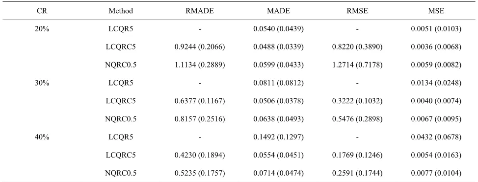
20% LCQR5 - 0.0540 (0.0439) - 0.0051 (0.0103)

LCQRC5 0.9244 (0.2066) 0.0488 (0.0339) 0.8220 (0.3890) 0.0036 (0.0068)

NQRC0.5 1.1134 (0.2889) 0.0599 (0.0433) 1.2714 (0.7178) 0.0059 (0.0082)

30% LCQR5 - 0.0811 (0.0812) - 0.0134 (0.0248)

LCQRC5 0.6377 (0.1167) 0.0506 (0.0378) 0.3222 (0.1032) 0.0040 (0.0074)

NQRC0.5 0.8157 (0.2516) 0.0638 (0.0493) 0.5476 (0.2898) 0.0067 (0.0095)

40% LCQR5 - 0.1492 (0.1297) - 0.0432 (0.0678)

LCQRC5 0.4230 (0.1894) 0.0554 (0.0451) 0.1769 (0.1246) 0.0054 (0.0163)

NQRC0.5 0.5235 (0.1757) 0.0714 (0.0474) 0.2591 (0.1744) 0.0077 (0.0104)

[image:4.595.54.541.545.731.2]

(5)

lung

log

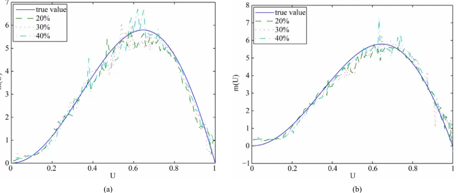
performance of LCQRC is presented in Figure 2. The

results of Example 1 and Example 2 show very similar messages.

the first one the mean absolute deviation error

3.3. Example 3

As an illustration, we now apply the proposed LCQRC to the lung cancer data. The data contain 228 observations on ten variables. The censoring percentage is 27%, so the estimators are expected to perform well. More details about the study can be found in [11], and the dataset is

included in the R package . We are interested in es-

timating the conditional of survival time (in days) given age (in years). Here, we use model (1) to fit the lung

cancer data, where is the ₁₀(survival time) and U

is the age/100. To evaluate the performance of our estimator. Two distance measures were approximated,

Y



MADEy



given by

1 1

ˆ

n i i i

y 







n y , and the second one



MSEy



defined as

the mean squared error





2 1

1 ˆ

n i i i

n y y 





, where n228. Furthermore, we de-

fine the rate of MADE_y and MSE_y which are

LCQR5

RMADEy MADE MADEy y and

LCQR5

RMSEy MSE MSEy y . Next, we report and com-

pare results with LCQR and NQRC for estimating the survival time. The simulation results for the LCQR,

LCQRC and NQRC are given in Table 5. It shows that

LCQRC is better than that of LCRQ and NQRC. Figure

3 summarize the simulation results for LCQRC5. It

(a) (b)

 

[image:5.595.73.531.297.490.2]

ˆ

Figure 1. Curve estimates of m  for Example 1. (a) n = 100; (b) n = 200.

(a) (b)

 

[image:5.595.70.531.519.715.2]

ˆ

(6)

Table 5. Simulation results of ˆy for lung cancer data.

RMADEy MADEy RMSEy MSE

Method y

LCQR5 - 0.6877 (0.7074) - 0.9711 (2.2640)

[image:6.595.72.534.104.675.2]

LCQRC5 0.9941 0.6836 (0.6788) 0.9536 0.9261 (2.0939) NQRC0.5 1.1172 0.7683 (0.5738) 0.9454 0.9181 (1.3586)

Figure 3. Curve estimates for lung cancer data.

shows that the proposal is valid.

4. Conclusion

In this work, we have focused on the LCQR for nonparametric model with censored data and its nice theoretical properties have been proven. The proposed appro- aches are demonstrated by simulation examples and real data applications. In addition, we believe the method can be extended to varying coefficient model (see [7]).

REFERENCES

[1] J. L. Powell, “Least Absolute Deviations Estimation for the Censored Regression Model,” Journal of Economet- rics, Vol. 25, No. 3, 1984, pp. 303-325.

doi:10.1016/0304-4076(84)90004-6

[2] S. Portnoy, “Censored Regression Quantiles,” Journal of the American Statistical Association, Vol. 98, No. 464, 2003, pp. 1001-1012. doi:10.1198/016214503000000954

[3] L. Peng and Y. Huang, “Survival Analysis with Quantile Regression Models,” Journal of the American Statistical Association, Vol. 103, No. 482, 2008, pp. 637-649.

doi:10.1198/016214508000000355

[4] H. J. Wang and L. Wang, “Locally Weighted Censored Quantile Regression,” Journal of the American Statistical Association, Vol. 104, No. 478, 2009, pp. 1117-1128.

doi:10.1198/jasa.2009.tm08230

[5] H. Zou and M. Yuan, “Composite Quantile Regression and the Oracle Model Selection Theory,” Annals of Sta- tistics, Vol. 36, No. 3, 2008, pp. 1108-1126.

doi:10.1214/07-AOS507

[6] B. Kai, R. Li and H. Zou, “Local Composite Quantile Regression Smoothing: An Efficient and Safe Alternative to Local Polynomial Regression,” Journal of the Royal Statistical Society, Series B, Vol. 72, No. 1, 2010, pp. 49- 69. doi:10.1111/j.1467-9868.2009.00725.x

[7] B. Kai, R. Li and H. Zou, “New Efficient Estimation and Variable Selection Methods for Semiparametric Varying- Coefficient Partially Linear Models,” Annals of Statistics, Vol. 39, No. 1, 2011, pp. 305-332.

doi:10.1214/10-AOS842

[8] R. Jiang, Z. G. Zhou, W. M. Qian and W. Q. Shao, “Sin- gle-Index Composite Quantile Regression,” Journal of the Korean Statistical Society, Vol. 3, No. 3, 2012, pp. 323-332. doi:10.1016/j.jkss.2011.11.001

[9] R. Jiang, W. M. Qian and Z. G. Zhou, “Variable Selection and Coefficient Estimation via Composite Quantile Re- gression with Randomly Censored Data,” Statistics & Probability Letters, Vol. 2, No. 2, 2012, pp. 308-317.

doi:10.1016/j.spl.2011.10.017

[10] A. Gannoun, J. Saracco, A. Yuan and G. Bonney, “Non- Parametric Quantile Regression with Censored Data,” Scandinavian Journal of Statistics, Vol. 32, No. 4, 2005, pp. 527-550. doi:10.1111/j.1467-9469.2005.00456.x

[11] C. L. Loprinzi, et al., “Prospective Evaluation of Prog-nostic Variables from Patient-Completed Questionnaires. North Central Cancer Treatment Group,” Journal of Cli- nical Oncology, Vol. 12, No. 3, 1994, pp. 601-607. [12] W. Gonzalez-Manteiga and C. Cadarso-Suarez, “Asymp-

totic Properties of a Generalized Kaplan-Meier Estimator with Some Applications,” Journal of Nonparametric Sta- tistics, Vol. 4, No. 1, 1994, pp. 65-78.

doi:10.1080/10485259408832601

[13] K. Knight, “Limiting Distributions for L1 Regression Esti-

mators under General Conditions,” Annals of Statistics, Vol. 26, No. 2, 1998, pp. 755-770.

doi:10.1214/aos/1028144858

(7)

Appendix



 



0 0

k k k

nh a m u u c

Lemma 1. Assume assumption A1 hold. Then

 







0



0 0

1 4 2 _,

1 2

ˆ _supsup ˆ

log

t U p

F F F

O n

 



t U F t U

n 



where 001 4.

Proof. This follows directly from theorem 2.1 of [12]. Proof of Theorem 1 Let

 

   ,



 

0



h nh bm u v,  _{i k}_,



_kvx_i



nh,



0



i i

x  U u h,

 

 



 





0 0 0 0

0

i i i

k i

d u m U m u m u U u

c  U  u



   

 



Then ₁, , ,Λq v



 





 





 





 









 





 





0 , 0

ˆ ,

ˆ

1 , ,

k k

k i i k i i k i i k i

i k i i k i i k i i k i

L K F A U c d u A U c d u

F B U c d u B U c d u

                                   _

 

i

is the minimizer of the following criterion:

1 1 i i

k i  q n

n



where Ai Yi m U

 

i ,Bi Yi 

   m U and K_iK





U_iu₀



h







 













 





0

0 0 d ,

y

. To apply the identity ([13])

x y x y I x I x z I x z

        

_

  

 



 







 





 





, 0 0 0 ˆ , , d q n

i i k i k i k

i i k i

L K F I A U c d u

u t

U c d u

t I B U c d u

                             



dt     we have

 



 



 



, , 0 1 1 0 0

1 1 0

ˆ i k

n i i k i k i i k i k

k i

q n

i i k i i k i i i k i

k i

q n

K  F  I A  U c d u t I A  U c d

       

 

    

 



₁ ˆ_,



i k i

K  F  I B

 



₁ ˆ_,





 



i i k i i k i

K  F  I B  U c d u

   

,

1 1 0

i k q n k i   

 

1 1

k i







1n 2n 3n 4n.

L L L L

≅

Y

Since is any value sufficiently large to exceed all m U

 

i , 3 ,



1 i

 

Fˆ, k



k

1 1

q n n i i k

k i

L K    L₄_n 0

 

 



  and  ,

then ₁ ₃ _,



 



 

₀



1 1

ˆ ,

q n

n n i i k i k i i k i k k i

L L K  F  I A  U c d u 

   



      2 2 1 q k n n k L L  



  ,

 

_

_{ }

_

_

_{ }

_

2 0 1 0

ˆ , d

i k n k

n i i k i i k i i i k i

i

L K  F  I A  U c d u t I A  U c d u t

    

 

_       _





 

.

Denote , where

0 .





 



 







 





 



 



 



0 0 0 0 , , 1 .

i k i i k i

i i i k i i i i k i i i i i i

k

i i k

i i

0 , 1 ₁

i i i k i

,

F I A U c d u

i k

i i

   

I C m U U c d u T U c d u I C m U U T C

I F C F C                          

nditional independence of T and C given U, we have

m U

C





c d u

I C m U U c d u T

     



(8)







 



   













   

0

,

, , d .

t C U

G t U F t U

E I C t T C U E I C t P T C C U F s U g s U s

    _            



Therefore, , 1

E I C_ t Tt U_P C t U P Tt U _







 



 











 



   

 





_{ }



 



 

    0 0 0 0 0 0 0 , 1 1

1 1 d .

1

i k

i k i i k i

m U U c d

i k i k

m U U c d

k

d

F I A U c d u U

G m U U c d U F m U U c d U F s U g s U s

F s U I F s U g s U s

F s U

                           _            



By Lemma 1, we have

 





E 

 







 







 







 



, i k n

 















 





 







 







 







 

, , , 0 1 0 0 1 0 0 1 0 0

ˆ , , d

ˆ _d

d 1

i k

i i k i k i i k i i k

i

n

i i k i k i i k i i k

i n

i i i k i i k

i

i i i k i i k p

i

K E F F I A U c t I A U c U t

K E O F F I A U c t I A U c U t

K E I A U c t I A U c U t o

                          _     _                    

 



1 0. n 



Then, we can obtain   

 







 





 













 





 







 

 







, , 2 0 0 1 0 0 0 1 0 T 0 2 ˆ 0 1 , , . 0 2 i k i k k n E L_ U_

0

, d

, d 1

n

i i k i i k i i i k i

i n

i i k i i k i i i k i p

i

k

U k k

k

K E F I A U c d u t I A U c d u U t

K E F I A U c d u t I A U c d u U t o

f u v v

                  _       _    _       _      _ _   

 

 



 





 



 



 





 







 

, , 2 1 0 0 0 1 0 2 2 , 1 Var ˆ Var , ˆ 1 . i k i k k n n

i i k i i k i i i k i i

n

i i k i i k i i i k i i

n

i i k p i L U 0 0 2 d , d

K F I A U c d u t I A U c d

E K F I A U c d u t I A U c d u

o K o

                   _                   _  _  











u t U

t U   _{ }     _ _ _{ }  _{ }       _     _ _     _   _

So, we can obtain  2

 

0



1

0 2

k k

n U k

L  f u v 







T

2

0

, k,

k v       

  , then

 

1 1

0 k k,

ˆ_k  f_U u M

where



(9)

 

0

 

1

1 n _{ˆ ,}

k i k i k i i i

M u K F I Y m U U

nh     





_ 



  _i c_kd u_i

 

₀



_.

Note that the error is symmet s

1

0

q k k

c 





, then it follows that

ric, thu

 

0

 

0 1

ˆ

k

U m U

q

1 q _{ˆ .} k

nh m 



 

 

 



 

Since Eki



F₀,k



I Y



im U

 

i  U ci k



0, then

 



 















 





 









 



 



 

0

0 1

0 0

1

0 1

2 2

0 2 0

1

1 _{ˆ ,}

1

1 1

1 _.

2 k

n

i k i k i i i k i

i n

i i k i i i k i i i k i

i n

i i k p

i

U k p

E M u U

nh

K E F I Y m U U c d u U

nh

K E F I Y m U U c I Y m U U c d u

nh

K d u o

nh

f u h m u o h

   

   

 



 

 

 

 _     _

     

  



  



, U op 1

 _  _

 

So, we can obtain

 

1 0

1

0

1

ˆ 1 2

0 2 0

bias

2

1 1

ˆ

var .

q U

k k

k

p

f u

m u U E M U

q nh

m u U o

nh nh





   _ _

 

 

     _ _

  _ _



 h m u ,