Which Spouse First Decides in the Household? The Dynamics of Bargaining

Which Spouse First Decides in the Household?

The Dynamics of Bargaining

Joaquín Andaluz Funcia1, Miriam Marcén1, José Alberto Molina Chueca1,2 1

Departamento de Análisis Económico, Facultad de Economía y Empresa, Universidad de Zaragoza, Zaragoza, Spain 2

Institute for the Study of Labour-IZA, Bonn, Germany Email: [email protected], [email protected], [email protected] Received December 14, 2012; revised January 15, 2013; accepted February 16, 2013

ABSTRACT

This paper examines the effects of which spouse first decides in the intrahousehold decision on the time that each spouse devotes to the provision of a family good. Specifically, we adopt a dynamic approach by developing a super- game, with the status quo being sequential, to study the influence of the discount factor, which measures the importance of the future, on the set of sustainable agreements in intrahousehold bargaining. We first show that cooperation is eas- ily sustained. We then observe a positive relationship between the discount factor and the proportion of time that the follower devotes to housework, when focusing on sustainable agreements, with this finding being maintained even if the follower has higher wages than the spouse leader.

Keywords: Family Bargaining; Stackelberg Game; Family Good

1. Introduction

Although the comparative advantage of women in house- hold production may have explained specialization in the past, Becker [1], this traditional theory is unable to ex- plain the current empirical evidence on the contribution to housework. Despite the increase in female labor force participation and female human capital, specialization within the household has remained relatively unchanged, Aguiar and Hurst [2]. Many women choose working ar- rangements that are compatible with caring for their chil- dren. Hersch [3], and indeed, women who work more hours than their husbands outside the home, or those who have higher earnings than their husbands do relatively more housework, Akerlof and Kranton [4].

Bargaining theories also fail to predict these findings. Under this approach, it would be expected a more egali- tarian allocation of time within the household as female human capital increases. Even more recent works on bargaining models of family decision-making, which extend the one-period approach to a dynamic setting, pre- dict a reduction in the incentives to specialize in house- hold production, Lundberg and Pollak [5]. In this setting, a consumption-smoothing problem arises, which may lead to the inability of spouses to engage in inter-tem- poral agreements, and that could lead to an inefficient allocation of household resources. The problem here is that a credible promise to compensate family public good production with future consumption cannot be made. The

sustainability of family bargaining agreements in a dy- namic setting is also analyzed in Andaluz and Molina [6]. By considering the trigger strategy, Friedman [7], as a punishment scheme, they show that the spouse with the higher bargaining power has a greater incentive to reach an agreement.1 Since bargaining power is not the only relevant factor in a dynamic family decision-making pro- cess, we add to this work by analyzing the influence of the discount factor, which measures the importance of the future, on the set of sustainable agreements, and on the time that each spouse devotes to the provision of a family good.

Our paper builds on the work of Andaluz and Molina [6], with one important distinction: we extend the analy- sis of the dynamic aspects of the family bargaining proc- ess, developing a supergame in which the status quo is not only defined as non-cooperative, but also as seque- ntial. We suppose that the spouses play a non-coopera- tive Stackelberg game, where the leader decides, first, contributions to a certain quantity of provision of family good, and thereby sets restrictions for the follower.

In our paper, we first solve the one-shot game, a Stackelberg game, and we then use this as the state game of an infinitely repeated game. To choose among the multiple equilibria of the repeated game, we focus on sustainable solutions and we determine the efficient al- location by way of the symmetric Nash bargaining solu-

1_{Note that sustainability here means the absence of incentives to}

tion. Using methodologies similar to ours, other studies such as Espinosa and Rhee, [8], have examined the rela- tionship between a union and a firm by developing a su- pergame with a threat to return to a noncooperative Sta- ckelberg equilibrium.

How does a spouse become a Stackelberg leader or a Stackelberg follower? In the literature of the economics of the family, we find several examples of marital rela- tionships modeled as a Stackelberg game. Bolin [9,10] suggests that a wife may be a Stackelberg follower if she considers the decisions taken by her husband as a fait accompli. Bolin analyzes the division of family work as the outcome of a Stackelberg game, showing that not only comparative advantage but also dominance are im- portant factors in time allocation. Another argument is proposed by Elul et al. [11], who consider that the age difference between spouses gives the husband a time advantage in the sequential decision game of time alloca- tion, through an analysis of the gender wage gap. Beblo and Robledo [12] also study the wage gap, but jointly with the gender leisure gap, providing empirical evidence that husbands enjoy more leisure time, all other things being equal, than their wives. They explain this empirical finding as a result of the husband being the Stackelberg leader in a sequential private provision game. In our case, we could also consider a situation in which the household division of labor is affected by social norms. The pre- scription that women should do the work at home may alter the family decision-making process, since one spouse, normally the husband, can make a credible com- mitment to contribute no more than a possibly very small amount to the provision of a family good. Thus, this spouse, usually the husband, becomes a Stackelberg leader and the other spouse, the wife, becomes a Stackel- berg follower.

As regards the main results, we observe an increase in the set of sustainable agreements derived from the bar-gaining, in a family setting, when the discount factor is higher. Thus, cooperation is more easily sustained. We also study the impact of the discount factor on the gains to well-being derived from cooperation, in order to ana-lyze whether the leader or the follower has incentives to reach an agreement. Although, in this case, our results are ambiguous, we show that the time devoted by the leader to the production of the family good is a key ele-ment in determining the sign of the relationship between the welfare gains and the discount factor.

Focusing on the sustainable solutions, we examine the relationship between the discount factor and the time devoted to the provision of a family good. What is clearly observed is that the contribution of the follower to the family good is increasing with respect to the discount factor. Then, if the woman is the follower (for instance, she decides second because of the existence of social

norms), we would expect her contribution to a family good to be greater when the discount factor increases (when women place more value on the future), even if there are no differences in the wages for men and women.2 This prediction appears to be confirmed by current empirical research that finds that wives undertake larger shares of the housework, regardless of their earn- ings.

2. Preferences

We suppose that the utility of each agent takes the fol- lowing functional form (see Konrad and Lommerud [14]):

1 1 1 ; 2 2 2

u   x Q q u x  Q q (1)

where x1 w1



1q1



and x2 w2



1q2



, wj

 

0,1

represents the wage rate for agent j, xj indicates the private consumption of agent , represents the family good, Q q1

j j1, 2; Q

2, q

  with qj j

being the pro- portion of hours that agent devotes to the provision of this good.

The maximum time available for each spouse is nor- malized to 1. In line with Konrad and Lommerud [14], we suppose that individuals increasingly dislike spending more time on the production of the family good. The contribution to the family good not only reduces the time available to the labor market, but also has a psychology- cal cost, represented by an increasing and convex func- tion in each of these arguments



q q1, 2



 

, with  and  being greater than 1. The family good, , can in- clude any situation which requires the joint performance of the spouses, e.g., raising the children or the mainte- nance of the home, but it excludes the possibility that the provision of the family good would be obtained in the market. This assumption can be reasonable if it takes into consideration that, for some couples, the private provi- sion of family goods is not a substitute for their own contribution to the family good. (Though it is not the aim of this paper, our model can be extended by considering both kinds of provision of family goods).

Q

We choose this special functional form for simplicity, although we acknowledge that this form can be restric- tive. When the spouses act non-cooperatively, the provi- sion of the family good by both agents is strategically independent, even though their utilities are intertwined through the existence of a family good. Then, this speci- fication establishes the non-cooperative outcome as a benchmark for understanding the family decision-making process.

2_{The discount factor of the leader is not a key element in this analysis,}

3. The One-Shot Game

To analyze how the discount factor affects both the set of sustainable agreements and time that each individual devotes to the provision of a family good, we first solve the one-shot game, a Stackelberg game, and we then use this as the state game of an infinitely-repeated game, using reversion to this non-cooperative Stackelberg equi- librium as the punishment for deviators. To determine the optimum levels of consumption and the contribution to the family good among the multiple stationary paths of the repeated game, we focus on sustainable solutions and we determine the efficient allocation as a result of the symmetric Nash bargaining solution, (see De la Rica and Espinosa [15]).

In each period , the non-cooperative equilibrium is the outcome of a Stackelberg game, in which the leader (spouse 1) commits to a certain quantity of provision of family good, while anticipating the optimal contribution of the follower (spouse 2).

t

Applying the backward induction procedure, we begin by obtaining the equilibrium corresponding to spouse (the follower). Formally:

2





2 2

2 2 2

,

2 2 2

1 1

Max

s.to 1

x q u x Q q

x w q

q q        (2)

From here, we deduce the levels of consumption and the provision of the family good:

1 1 1 1

2 2

2 2 2

1 1

; 1

w w

q x w

                _{ }   _{ } 

      (3)

and the utility level:





1

2

2 2 1

1 1

d w

u w q

           _{  }

  (4)

For spouse 1 (the leader) we formulate the following maximization problem:





1 1

1 1 1 ,

1 1 1 2 2

Max

s.to 1

x q u x Q q

x w q

q q         (5)

and we obtain the level of private consumption, and the provision of the household good made by spouse 1:

1

1 1 1

1 1 1 1

1 1

; 1

w

q x w

            _{ }   _{ }    _   1 w      

solution for both spouses are:

(6)

Therefore, the levels of utility in the non-cooperative









1 2

1 1 2 1

1 1 1

1 w 1 w

, 1

u q q w

           _{  }    _        

  (7)









2 1

2 1 2 2

1 1 1

1 1

, 1 w w

u q q w

           _{  }           

    (8)

The solution obtained in (3) and (6), is an interior so- lu

ibutor.

tion.3 In addition, we may determine the situations in which only one of the spouses is the contributor to the family good, to see whether there is a dominant strategy (see Bucholz et al., [16]). We can distinguish two addi- tional Stackelberg equilibria:

The leader is the only contr

In this case, Q, the family good, is only supplied by

spouse 1, from (5) and with q20, we can obtain the

total family good:

1 1 1 .        : 1 w

Q   and the levels of utility of both spouses

 





 

1 1 1 1 1 2 2 1 1 1

, 0 1 ;

1 , 0

w

u Q w

w

u Q w

    _        _{  }            

The follower is the only contributor.

ouse 2,(2), and

w

From the maximization problem of sp

ith q10, we may determine the levels of provision

of family good which are only provided by spouse 2:

1 1

1w 

 2 _.

Q _{  }

 

_

with the levels of utility for both spouses in this case be- ing:

 

 





1 1 2 1 1 2 2 2 1 1 0, ; 1 0, 1 w

u Q w

w

u Q w

     _       _ _     _{  }        

Under the structure of preferences defined above, for all values of the parameters, the interior solution con- stitutes a dominant strategy for both agents in the Sta- ckelberg equilibrium.4 It is straightforward to deduce that

3_{Note that, under the preferences specified above, the reaction functions}

for both spouses have null slope, and thus, the provision of the family good by both agents is strategically independent. As a consequence, the levels of consumption and the provision of the family good obtained in the Stackelberg equilibrium coincide with those obtained in a Nash equilibrium.

4_{This result differs from that obtained by Bucholz et al. [16]. However,}





 

1 1, 2 i , 0

u q q   _u Q

and that

,



1, 2



 

0,

i i

u q q   _u Q







0 w_i 1;  , 1, i 1,

    

result, since we do not consider t



2 . This is a reasonable



he possibility that one spouse compensates the other.

However, the interior solution, the dominant strategy, is clearly inefficient, as can be seen in Figure 1 where it is represented the curves of indifference of the spouses in the non-cooperative solution. For spouse 1, the slope of the curve of indifference in the non-cooperative equili- brium is zero in



q q1, 2



,

 

and is increasing and convex

if q1q1 and q2 q2,

1

2

d

0

q _

, 1

dq _u

1

2 2

d

0

q _

. Ana-

2 1

dq _u

logously, for spouse 2, the slope of the curve of indif- ference that contains the solution of the one-shot game is equal to minus infinity in the combination



q q1, 2



  , and is increasing and concave when q1 q1



 and q2 q2,





2 2

2

2 2

d d

0; 0.

q _ q _

All the poi ated in

2

1 1

dq _u dq _u

nts loc side the

area formed by both curves of indifference are Pareto

4. Dynamic Setting

y-repeated game, in which the superior to the equilibrium of the one shot game, as Kapteyn and Kooreman [17] demonstrated. Those points located in the contract curve CC’ are efficient solutions.

We consider an infinitel

two members of a family, spouse 1 and spouse 2, may contribute voluntarily to the provision of a family good whose consumption is non-rival, as in [3]. We suppose that the spouses do not know the moment of the dissolu- tion of the marriage, and that the objective of each is to

Iso-g

C’

0 _q* _q1

1

q*2

q2

C

Iso-u* 1

[image:4.595.66.275.540.724.2]

Iso-u*2

Figure 1. Set of Pareto-Superior Solutions.

maximi ilities.5

where

ze the discounted value of their current ut Formally:









1 1

, ; 1, 2

t

j j

t

u x Q j

 









 

0,1



ents.

denotes the discount factor, common to

ficient equilibrium in a dy- na

cus on stationary pa

is both ag

Is it possible to reach an ef

mic setting? When the decisions are taken in a multi-period framework, the loss from non-cooperation accumulates, and strong incentives appear to reach a Pareto Superior agreement. However, repetition alone is not enough to eliminate the non-cooperative static equili- brium, and thus the one-shot Stackelberg equilibrium is another possible outcome of the repeated game. To arrive at a combination that is Pareto superior to the one-shot non-cooperative equilibrium, it is necessary that both spouses implicitly create a credible strategy that deters deviations from a cooperative solution. As in Andaluz and Molina [6], we consider the so-called trigger strategy (Friedman [7]). In this case, when there is a deviation from the cooperative solution, the levels of private con- sumption, and the provision of the family good revert to those of non-cooperative equilibrium. The threat of re- taliation, through reversion to this punishment path, sus- tains Pareto Superior outcomes and is credible, since it is in the best interest of each agent not to deviate unilater- ally from the cooperative equilibrium.

For the sake of simplicity, we fo

ths for all t. In a subgame perfect equilibrium, a sta-tionary path sustainable if it satisfies the following conditions:



,



0;

i i i

u x Q _u_ i_{1, 2}

(9)





_{ }

2 2 2

2 1

, 1

d

u x Q u

u q

1



 



 

  (10)

Condition (9) establishes that both spouses have in- centives to cooperate, since the well-being these agents obtain in the cooperative solution is greater than, or equal to, the well-being obtained in the non-cooperative solu- tion. Condition (10) determines that the spouse who de- cides second has no incentive to deviate from the effi- cient solution.Condition (9) is not enough to obtain sta- tionary paths, since the follower, given q1, could react by deviation to maximize his/her own utility. To solve this problem, it is necessary to introduce inequality (10), which states that the discounted value of the well-being of the follower, conforming to the specified path, the left-hand side of the inequality, is greater than the well-being from the optimal one-shot deviation and the subsequent reversion from the following period, onwards

5_{Our approach is developed in an environment where marital partners}

to the punishment path, the right-hand side of the ine- quality.6

In this setting, the maintenance of the cooperative equilibrium depends on the agent who decides second. If spouse 1 deviates from a cooperative agreement, this is immediately observed by spouse 2, thus eliminating any possible short-term well-being ains for spouse 1. Moreover, the leader’s discount rate plays no role, since the one-shot game is sequential. However, the follower’s discount rate is a key element in the maintenance of the cooperative solution.

Unless

g

 is very high, constraint (10) is always binding in equilibrium, whereas (9) is not. Denote  the minimum value of discount factor for which (10) not binding, and let the function g g q q



1, 2,



is 

 rep-

resent the long-term gain from the follower’s cooperation determined from (10). Formally:













1 1 1

1 2

2 2 2 1

2 1

, ,

g q q 

1

1 1

1

w q q q

w  w 

 _

 

 

 

   

   

 

  _{    }

   

(11)

When q1 q1 and 

 q2 q2



 , the function g is in- creasing a cave, with t value of its slope being minus infinity in the non-cooperative solution

nd con he



q q1, 2



  . The function g is represented by a broken lin - ure 1. Among e Pareto-superior combinations

e in Fig

th



q q1, 2



,

which are those points located in the contract curve CC’, the function g allows us to identify a subset of sus- tainable solutions, all the combinations of



q q1, 2



lo-

cated to the right of the dashed line, wh be achieved by way of repeated interaction. This subset of Pareto-superior solutions to the equilibrium of the one- shot game is greater when the discount factor is higher, since the function

ich can

g is increasing in . Thus, coop- eration is more easily sustained as  increases.

5. Bargaining Solution

le equilibrium among the In order to determine a sing

multiple stationary paths, we suppose that there exists a bargaining process, not modeled explicitly here, and as a result, both spouses take their decisions by way of the symmetric Nash bargaining solution.7 Focusing on the sustainable solutions, spouses choose the stationary paths of private consumption and family good provision that

maximize the product of the utilities, after being normal- ized by the utility levels of the non-cooperative solution. Formally, the problem becomes, for   













1 2 1 2

1 2 1 2 1 1 2 2 , , ,

1 2

Max , , ,

s.to , , 0

x x q q J x x q q u u u u



g q q 

 

  

 (12)

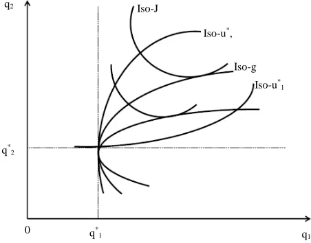
When  takes value zero, the non-cooperative solu- tion satisfies restrictions (9) and (10). Alternatively, if this factor takes value one, all the Pareto-superior solu- tions are indeed sustainable and, consequently, the bar- gaining agreement constitutes an efficient solution. Be- tween these two extremes, the solution of the previous problem depends on the discount factor through con- straint g q



1,q2,



0. The bargaining solution is de-

termined by way of the tangency between an Iso-J line and an Iso-g line, as shown in Figure 2.8

Under some regularity assumptions (see Appendix) we obtain the following proposition:

Proposition 1.

For   

The contribution to the family good of the spouse who decides second (follower) is increasing with respect to

the discount factor: d 2 _0.

d

q

 

The influence of the discount factor on the contribu- tion to the family good of the spouse who decides first

(leader) is ambiguous: d 1 ₀

d

q

  or 1

d 0 d

q

  .

Proof. (See Appendix).

This proposition indicates that the agent who decides second will devote more time to the provision of the family good when he/she values the future heavily (a

q*1

0 _q

1

q2

q* 2

Iso-J

Iso-u*_,

Iso-g

Iso-u* 1

6_{This is not applicable to the situation of the standard case of Nash}

reversion, since, in this situation, decisions are taken simultaneously, and to obtain stationary paths it is necessary to include an additional inequality similar to that introduced for spouse 2, (10), but in this case it must also be established for spouse 1.

7_{This solution implicitly assumes a bargaining process resulting in the}

[image:5.595.309.535.499.676.2]

generalised bargaining solution (see Binmore et al. [18]; Harsanyi [19]).

Figure 2. Set of possible sustainable bargaining solutions.

8_{It is straightforward to deduce that under the structure of preferences}

high discount factor). However, the path of the contri- bution to the family good made by the spouse who de- cides first can be increased or decreased. An increasing evolution would imply that the difference between the hours this agent devotes to the family good in the coop- erative solution, and the hours determined in the non- cooperative equilibrium, will not be significant.

Note that we have found that the discount factor can increase the provision of the family good without im- posing any restriction on the follower’s relative earnings, or on the psychological cost produced by devoting time to the family good. Thus, if the woman is the follower, the higher the discount factor, the higher the provision of the family good, even with the wage rate being the same for both spouses.

For the leader, spouse 1, we find a subset of sustain- able solutions where the spouse who decides first in- creases or decreases provision of the family good, de- pending on the discount factor. There exists a level of provision of the family good, qˆ ,1 with qˆ1 q1,





q

which represents the minimum value from which the relation- ship between the discount factor and the level of provi- sion of the family good made by this agent becomes negative. By contrast, for 1 1 1 when the dis-

count factor increases, the provision of the family good by the leader increases. Thus, situations in which the husband devotes much less time to the family good than does the wife can be possible sustainable agreements, even without differences in the salaries of the spouses, as a resultof a high discount factor.

ˆ

 

q q

The discount factor also reflects the subjective proba- bility that the game will end. The higher the discount factor, the lower the probability that the game will end in the near future. Even when there is a possibility that the game will end sometime in the future, as in the case of intertemporal agreements within the family subject to renegotiation, our optimum provision of the family good can support a near-efficient outcome, as long as each spouse believes, with a high enough probability, that the game will continue. Thus, although we have considered an infinitely repeated game, it is possible to make agree- ments in a dynamic setting with a finite horizon (see Espinosa and Rhee [8]).

Knowing the evolution of the paths of the provision of the family good, we can deduce the influence of the dis-count factor on the level of utility derived from the co-operation.

Corollary:

For   

In the bargaining solution, a variation of the discount

factor can increase or reduce the levels of utility for both spouses: d 1 _0;d 1 _0;d 2 _0;d 2 ₀

d d d d

u u u u

       

Proof. (See Appendix).

Specifically, we observe that, for 1 1 when the discount factor increases, the provision of the family good by the leader decreases, generating opposite effects on the level of utility of the spouses. The level of utility increases for the leader and decreases for the follower. By contrast, for 1 1 1

ˆ

q q

ˆ

q_q _q

when the discount factor increases, the provision of the family good by the leader increases, and the levels of utility can increase or de- crease for both spouses.

6. Conclusions

Family bargaining models have usually presented the household allocation problem in a static setting. However, households endure for more than a single period, which can potentially, and substantially, affect the family deci- sion-making process and it is thus necessary to view bargaining in a multi-period context.

In this dynamic setting, we have set up a supergame in an intrahousehold framework, in which both spouses may contribute voluntarily to the provision of a family good. Assuming that the status quo is not only defined as non-cooperative, but also as sequential (equilibrium of Stackelberg), and that the efficient allocation is given by way of the symmetric Nash bargaining solution, we de- duce the influence of the discount factor on the sustain- ability of agreements, and on the time that each individ- ual devotes to the provision of the family good. We ac- knowledge that we have not included all the factors that affect the dynamics of intrahousehold bargaining, and some of our assumptions are potentially restrictive, but we view this work as a benchmark for understanding long-term marital relationships.

The following conclusions are obtained. First, the set of possible sustainable agreements derived from bar- gaining is greater when the discount factor of the spouse who decides second is higher; cooperation is more easily sustained. However, it is not clear whether a greater dis- count factor increases the incentives to make an agree- ment, since we show that the discount factor has an am- biguous impact on the gains of well-being derived from the bargaining. The effect of the discount factor will be positive or negative, depending on the increase in the time devoted by the leader to the production of the fam- ily good in the bargaining solution.

for both spouses.

7. Acknowledgements

Support from the Spanish Ministry of Economics is gra- tefully acknowledged (grant reference number ECO2012- 34828).

REFERENCES

[1] G. S. Becker, “A Treatise on the Family,” Enlarged Edi-tion, Harvard University Press, Cambridge, 1991. [2] M. Aguiar and E. Hurst, “Measuring Trends in Leisure:

The Allocation of Time over Five Decades,” The Quar-terly Journal of Economics, Vol. 122, No. 3, 2007, pp. 969-1006.doi:10.1162/qjec.122.3.969

[3] J. Hersch, “The Impact of Nonmarket Work on Market Wages,” American Economic Review Papers and Pro-ceedings, Vol. 81, 1991, pp. 157-160.

[4] G. Akerlof and R. Kranton, “Economics and Identity,” Quarterly Journal of Economics, Vol. 115, No. 3, 2000, pp. 715-753.

[5] S. Lundberg and R. A. Pollak, “Efficiency in Marriage,” Review of Economic of the Household, Vol. 1, No. 3, 2003, pp. 153-167.doi:10.1023/A:1025041316091

[6] J. Andaluz and J. A. Molina, “On the Sustainability of Bargaining Solutions in Family Decision Models,” Re-view of Economics of the Household, Vol. 5, No. 4, 2007, pp. 405-418.

[7] J. Friedman, “A Non-Cooperative Equilibrium for Su-pergames,” Review of Economic Studies, Vol. 38, No. 113, 1971, pp. 1-12.

[8] M. P. Espinosa and C. Rhee, “Efficient Wage Bargaining as a Repeated Game,” Quarterly Journal of Economics, Vol. 104, No. 3, 1989, pp. 565-588.

[9] K. Bolin, “An Economic Analysis of Marriage and Di-vorce,” Lund Economic Studies, University of Lund, Lund, 1996, p. 62.

[10] K. Bolin, “A Family with One Dominating Spouse,” In: I. Persson and C. Jonung, Eds., Economics of the Family and Family Policies, Routledge, New York, 1997, pp. 84-99.doi:10.4324/9780203441336.ch4

[11] R. Elul, J. Silva-Reus and O. Volij, “Will You Marry Me? A Perspective on the Gender Gap,” Journal of Economic Behaviour and Organization, Vol. 49, No. 4, 2002, pp. 549-572.doi:10.1016/S0167-2681(02)00006-9

[12] M. Beblo and J. R. Robledo, “The Wage Gap and the Leisure Gap for Double-Earner Couples,” Journal of Population Economics, Vol. 21, No. 2, 2008, pp. 281- 304.

[13] D. J. Benjamin, J. J. Choi and A. J. Strickland, “Social Identity and Preferences,” American Economic Review, Vol. 100, No. 4, 2010, pp. 1913-1928.

[14] K. A. Konrad and K. E. Lommerud, “The Bargaining Family Revisited,” Canadian Journal of Economics, Vol. 33, No. 2, 2000, pp. 471-487.

[15] S. De la Rica and M. P. Espinosa, “Testing Employement Determination in Unionised Economies as a Repeated Game,” Scottish Journal of Political Economy, Vol. 44, No. 2, 1997, pp. 134-152.

[16] W. Buchholz, K. A. Konrad and K. E. Lommerud, “Stackelberg Leadership and Transfers in Private Provi-sion of Public Goods,” Review of Economic Design, Vol. 3, No. 1, 1997, pp. 29-43.

[17] A. Kapteyn and P. Kooreman, “On the Empirical Imple-mentation of Some Game Theoretic Models of Household Labor Supply,” The Journal of Human Resources, Vol. 25, No. 4, 1990, pp. 584-598.

[18] K. Binmore, A. Rubinstein and A. Woolinsky, “The Nash Bargaining Solution in Economic Modeling,” Rand Jour-nal of Economics, Vol. 17, No. 2, 1986, pp. 176-188. [19] J. C. Harsanyi, “Rational Behaviour and Bargaining

Equi-libria in Games and Social Situations,” Cambridge Uni-versity Press, Cambridge, 1977.

Appendix

Proof of Proposition

To be able to characterize the solution of the maxi- mization problem proposed in (12), we introduce the fol- lowing assumptions:

We suppose that J x x q q



1, 2, 1, 2





, , ,

is strictly concave. The level curves of J x x q q1 2 1 2



are monotone:



1 2



1 0 J J q  

 (13)

For q10,q20, the first order conditions are:

1 1 0

J g 

2 2 0

J g 



1, 2,



0

g q q  

with  0, the multiplier of the problem of maximiza- tion. Thus, it is possible to deduce the following equation:

1 2 2

1

J g

J  g (14)

Differentiating with respect to  , we obtain that:





1





2

11 11 12 12 1 1

d d _d

d d d

q q

J g _  J g _ g _  g_





1





2

21 21 22 22 2 2

d d _d

d d d

q q

J g _  J g _ g _  g_

1 2 1 2

d d

d d

q q

g _ g _  g_

These equations can be written in matrix form as:



 





 



1

11 11 12 12 1 1 2

21 21 22 22 2 2

1 2 d d d d 0 _d d q

J g J g g g

q

J g J g g g

g g  g        _                 _{ }  _{ }    _{ } _  _{    }  _{ }     

The matrix on the left hand side is the bordered Hes-sian. Applying Cramer’s rule it is possible to obtain the changes in q2 when  changes:







11 11



1 1

2

21 21 2 2

1

d 1

d

0

J g g

q g

J g g

D g g              

g (15)

where D is the determinant of the bordered Hessian. The second order conditions of the maximization problem require that D be positive.

Therefore, the sign of d 2

d

q

 is determined by the sign







 







1 2 2 2 1 1 1 11 2 2 12

d

sign sign 1

d

1

q

w q

q q J w q J

           _{   }   _         _ (16)

Given that



1



2 2 2 2

1w q  0 q q,and under (13) and (14), we deduce that (16) is positive: dq2 _0.

d

t to δ, we ha

Differentiating the restriction with respec ve:



 

1



1 2

1 1 2 2

d 1 d

1

d d

q q

q q w q

  

 

 

  _     _

  (17)

Thus, the sign of d 1

d

q

 is the sign of the numerator:



 

1



1 2

1 1 2 2

d d

sign sign 1

d d

q q

q q w q

   

 _ _{    }

   

   

Given that



 

1



2

1 1 2 2

d

0, 1 0 0,

d

q q q  w q   _ 

we deduce that

1

d 0. d

q

  or 1

d 0. d

q

 

From (15) and (17), we can determine a value qˆ1, with

1

ˆ

q q₁, which represents the minimum value from e relationship between the discount factor and the level of provision of the family good made by this agent becomes negative. So, when q1qˆ1, we obtain that which th 1 d 0 q

d  and when qˆ q q



 

1 1 1 what we obtain

is that d 1 _0.

d

q

 

f of Coro ry

ope theorem, we derive the utility fu

Proo lla

Applying the envel

nction of both spouses with respect to :

For spouse 1, we obtain:

1 1 1 1

1 2

2

d

d d

d

q u q

q q

du u d

 





 

  (18)

Taking into account (17), this expression takes the fol-lo  wing form: of (15):













1

1 1 1 1 1

1 1

1 1 2 2 ₂

d

1 1 _d

1

d

w q q q

w q w q _q



1







1 1

1w q 0, 1 2

2 2

d

1 0,

d

q

w q _

   0,



q1 q1



0,



  0  1, 0q_i1



i1, 2 ,



we de- duce that: d 1

0 d

u

  or

1 0  d

d

u



Analogously, given that d 2 ₀

d

q

  and with 1

d 0 d

q

  ,

we obtain that du1 0

d  with q1qˆ1. When

1

d 0 d

q

  ,

we obtain that d 1 0 d

u

  with .

,

1 1

ˆ

q q q₁ For spouse 2

2 2 1 2

1 2

d d

d d

d

u u q u q

q q

 



₁





1 1



2 2

2 2

d ₁ d

1 1

d d

q q

u q

w q

 

 



 

     .

Analogously, we obtain that



1



2 2

2 2

d d

1 .

d d

d

u q

w q dq1

 





   

Given that d 2 ₀

d

q

  and with 1

d

0, we obtain

d

q

 

that d 2 _0.

d

u

  Remember that it is necessary that q1qˆ1 to obtain a negative relationship between the discount factor and the level of provision of the family good made

by spouse 1. When d 1 ₀

d

q

  , we obtain that d_du2 0, with qˆ1 q1 q1



  . 2

d

 



 

 

 