Munich Personal RePEc Archive
Exchange Volatility and Export
Performance in Egypt: New Insights
from Wavelet Decomposition and
Optimal GARCH Model
Bouoiyour, Jamal and Selmi, Refk
CATT, University of Pau, ESC, High school of trade of Tunis
2013
Online at
https://mpra.ub.uni-muenchen.de/53106/
1
Exchange Rate Uncertainty and Export Performance in Egypt:
New Insights from Wavelet Decomposition and Optimal GARCH Model
Prepared by:
Jamal Bouoiyour a and Refk Selmi b1
a CATT, University of Pau, France.
b ESC, High School of Trade of Tunis, Tunisia.
Abstract: To assess the link between exchange rate uncertainty and exports performance in
Egypt, this article relies on an optimal GARCH model chosen by information criteria among decomposed series on a scale-by-scale basis (wavelet decomposition). The observed outcomes reveal that this relationship depends intensely on the frequency-to-frequency variation and slightly on the leverage effect and switching regime. Indeed, it is well shown that at the low frequency, the coefficient associated to exchange rate volatility’s effect on exports is greater than that at the high frequency and conversely when subtracting energy’s share. We attribute the apparently conflicting results to the co-movement between energy prices and those of other commodities, the excessive speculation and the composition of trade partners.
Keywords: Exchange rate uncertainty; exports; wavelets; optimal GARCH model.
1 Corresponding authors: CATT-UPPA, Avenue du Doyen Poplawski BP 1633, 64016 Pau, Cédex.
Tel : (33) 5 59 40 80 01
2
1.
Introduction
The relationship between exchange rate uncertainty and exports performance has been investigated in several researches but no consistent results have been up to now found. The subject on how the exchange rate volatility impacts trade has been investigated and the results have varied widely. Some studies have found a negative interaction between currency risk and exports (e.g. McKenzie (1998), Vergil (2002), Nabli and Varoudakis (2002),
Bahmani-Oskooee (2002) and Rey (2006), etc…). Others have found that higher risk associated with
ups and downs exchange rate’ movements can lead to great opportunity increasing exports performance (e.g. De Grauwe (1992) and Achy and Sekkat (2003), among others). More recently, Egert and Zumaquero (2007), Bouoiyour and Selmi (2013) argue that there is an ambiguous effect.
These empirical studies suggest that the link between exchange rate uncertainty and trade performance varies depending on risk-averse, the absence of hedging instruments, the specialization and the degree of competitiveness. To reconcile the mixed results of prior researches, using meta-regression analysis, Coric and Pugh (2010) provide evidence that the effect of exchange volatility on trade is likely to be adverse when measured in real rather than nominal term and when less developed rather than developing countries are considered.
Despite the many studies on this subject and the different estimation techniques used, analytical gaps remain, especially methodological ones. To contribute to this literature stream and while trying to highlight additional explanations of the conflicting results, we extend our examination beyond by assessing this link depending to frequency-to-frequency variation.
Alternatively, various questions can be raised. For example, To what extent exchange rate uncertainty affect Egyptian exports? Do exports react differently when moving from one frequency band to other? How to choose the optimal model to determine volatility?
The answers of these several questions will enhance our understanding on the relationship between exchange rate volatility and exports performance in Egyptian case and allow us to identify the main sources behind the study-to-study variation related to the focal linkage.
3
we estimate the linkage between real exchange rate volatility and real exports returns using wavelet decomposition and an optimal model among several GARCH extensions chosen by various information criteria. Additionally, we discuss our main results. Section 5 concludes.
2.
A brief overview of exchange and trade policies in Egypt
Since the demise of the Bretton Woods system in 1973, particularly early 80’s, Egypt
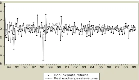
had a fixed system of its currency in relation to U.S. dollar. With the beginning of the economic reform program in 1991, government announced the adoption of managed floating regime (e.g. Kandil and Nergiz, 2008). From 1997, the Egyptian exchange rate has undergone numerous shocks such as the East Asian crisis and Luxor terrorist attack in 1997, the fall of oil prices in 1998 and the revival of tensions in the Middle East peace process in the end of 90’s. These latter led to capital outflows, a slowdown in the capital market, a deterioration of the current account balance and a slowdown in tourism sector and economic growth. At this period, International Monetary Fund ranked Egypt as having conventional fixed peg (e.g. Kamar, 2004). In order to mitigate exchange rate-damaging, the Central Bank of Egypt decided to restore market stability by introducing a crawling peg system. This exchange regime allows the nominal exchange rate to move in a band within upper and lower limits. As a result, it is seen from the Figure 1, a real depreciation of Egyptian pound. Unfortunately, the aftermath of the New York terrorist attack and the subsequent wars on Afghanistan and Iraq
darkened the investment’s attractiveness of Egypt. All the above events put Egyptian pound
under pressure.
Between 1995 and 2009, real exports exhibited great instability (see Figure 2). The World Trade Organization agreement signed with the European Union in 1995 allowed Egypt to develop its export competitiveness, improve its comparative advantages and provide a greater access to developing markets with growing concern for manufactured sector (e.g. Nabli and Varoudakis, 2002). This reform led it to consolidate its position in foreign trade during the period from 1996 to 2004 (e.g. Sekkat, 2012). However, the dismantling of the textile and clothing agreement and the accession of China into the World Trade Organization have degraded the position of this sector compared to previous years.
4
products’diversification, i.e. the diversification on non-oil sectors can limit real exchange rate appreciation (e.g. Espinoza and Prasad, 2012) ; (ii) an integration in international financial market allowing this country to smooth the adjustments of primary commodity prices and reduce costs of volatile exchange rate on exports performance (e.g. Gourinchas and Rey, 2007) ;(iii) more credible monetary policy to absorb several shocks and then to remedy an overvaluation of real exchange rate.
3.
Wavelet decomposition and optimal GARCH model
Since the majority of researches on the link between exchange rate volatility and exports performance were always contradictory and inconclusive, this study seeks to clarify the inconsistent results. In so doing, we assess differently the relationship between changes in
real exchange rates and those of real exports in Egypt using wavelet decomposition and
optimal GARCH model2.
3.1. Why wavelets?
Wavelets are “small waves” that grow and decay in a limited time period. Wavelet analysis involves the projection of the original series into several frequencies by separating each series into its constituent frequency components. This technique is a decomposition of time series into high frequency or noisy components and low frequency or trend components. Wavelet method allows us to extract the various time scales driving any macroeconomic variable in the time domain by decomposing it into its frequency band components. This can reflect structural changes that can happen over time and at a well-defined time scale.
This approach is based on the mother wavelet denoted
(
t
)
, which must satisfy:1 ,
0 )
(
2
t dt
dt (1)To quantify the importance of the wavelet decomposition into various frequencies, the
mother wavelet
(
t
)
gets deleted, so:
s
u
t
s
s
u
,1
(2)
5
where u and s are the time location and frequency ranges, respectively, and
s
1
indicates that
the norm of
u,s(
t
)
is equal to unity.The wavelet decomposition in turn is a succession of low and high-pass filters of the focal series. Unlike time domain analysis, wavelets can identify which frequencies are present in the data at any given point in time. Ultimately, we obtain the following wavelet
representation of the function X(t):
(
),
(
),....,
(
),
(
)
)
(
t
w
1t
v
1t
w
t
v
t
X
j j (3)where w1(t) and v1(t) respectively wavelet high frequency and wavelet low frequency.
Considering several frequency bands, time series can be extracted for further analysis. Firstly, with wavelets analysis, we can differentiate between time periods for decision making. Secondly, since wavelets method enables to decompose a signal into multi-resolution components, it allows us to assess both real exchange rate and real exports data over well- defined time horizons. Thirdly, with this technique, we can approximate structural changes that can happen over time. Finally, the problem of temporal aggregation bias can be neglected because time series were decomposed into different time scales. Therefore, wavelets analysis provides a fresh look into the link between exchange rate uncertainty and exports performance by highlighting it over different and precise horizons.
3.2. Why GARCH models?
While modeling strategies have evolved over time to incorporate new developments in econometric analysis, no single measure of exchange volatility has dominated the literature (e.g. Haile and Pugh, 2011).
6
In this study, we use 13 GARCH extensions while trying to choose the best model that can captures more how behave real exports after changes in real exchange rate. With regard to these various specifications, it is of utmost importance to evaluate whether changes in real exchange rate have temporary, permanent, transitory, asymmetrical or nonlinear effects on real exports performance. Therefore, we seek to examine if: (i) First, volatile supply leads to changes in demand conditions and thereby to multiple commodity price regimes. This yields to take into account the threshold effect in the focal linkage; (ii) the possible intervention of monetary authorities in exchange market leads us to take into account good and bad news and
not only the magnitude of shock; (iii) the exchange rate volatility’s effect on exports can be
transitory or permanent. Thus, it seems appropriate to decompose the impact of changes in real exchange rate and those of real exports into a long run time varying trend and short run transitory deviations from trend.
3.3. Data sources and methodological framework
A central goal for this study is to check if the connection between real exchange rate uncertainty and real exports varies over time (i.e. from low to high frequency bands). We estimate various GARCH extensions and seek the optimal model that can best capture a significant relation on the basis of an historical evaluation. Intuitively, we explore a bivarite
GARCH model3 without taking into account other determinants of exports because instead of
analyzing the effects of its fundamentals, as it is usually done (e.g. Achy and Sekkat (2003), Rey (2006), Egert and Zumaquero (2007), among others), we decompose here the two key variables at various scales of resolution using wavelet decomposition and then we study the focal relationship among the decomposed series matched to their scales.To do so, we built an indicator that replaces the simple changes of real exports in accordance with real exchange rate returns. This indicator is constructed using the variance between both variables in question.
We use monthly data for the period from 1994 to 2009 collected from EconstatsTM and
International Monetary Fund (IMF). Thus, we consider the following variables:
r XPRt = log (XPRt/XPRt-1) (4)
where r XPR t is the return of real exports determined using the ratio between nominal exports
and the export unit value.
3 This method has been largely used recently to evaluate the link between the variability of dollar vis-à-vis
7
r REERt = log (REERt/REERt-1) (5)
where r REER t is the return of real exchange rate. The real exchange rate is constructed by
dividing the trade-weighted foreign price level index by the corresponding domestic price level index, after converting the values to a common scale using nominal exchange rate.
REER t=NEER t (P*t/Pt) (6)
To assess this link between real exchange rate returns and those of real exports under
different time scales, we begin by a linear model which is forward looking at time t.
rXPRt
rREERt
t (7)where
t is the error term.Thereafter, we applied GARCH model chosen depending to frequency-to frequency variation. It is of course shown that GARCH-type modeling allows us to have several results (e.g. Anderson et al. 2009). The unobserved conditional variance has affected widely the development of various GARCH-type models (e.g. Engle, 1982). Several specifications have been advanced to capture different features that are thought to be important. For instance, some GARCH extensions allow the volatility to react asymmetrically to positive and negative shocks (e.g. Nelson, 1991), others consider only the magnitude of shocks (e.g. Bollerslev, 1986). This has created a need to understand clearly if the performance of GARCH models varies over time. Accordingly, a large strand of literature on financial engineering has attempted to check whether GARCH models vary depending to time periods (e.g. Engle et al. (1987), Tong (1990), Bollerslev et al. (1993), Bera and Higgins (1993), Campbell and Mackinlay (1997), Hansen (2001), among others).
The common conclusion is that across different time periods, there is a change in volatility’s behavior over time, leading to a change in GARCH parameters. More precisely, the model is capable of accommodating systematic changes in the amplitude of the volatility clusters that cannot be explained by a constant-parameter GARCH model. Recently, Mazur and Pipien (2012) show that Financial markets data often exhibit volatility clustering and cyclical behavior, where time series show periods of high volatility and periods of low volatility.
8
summarizes their expressions. These criteria evaluate the models based on the historical volatility. The discrimination function differs from one test to another. There is not really an optimal model but the optimality remains concerning the choice of the test. These criteria seem sufficient to judge the quality of the estimation (e.g. Bouoiyour et al. 2012).
4.
Application and main findings
4.1. Preliminary analysis
We report the descriptive statistics in Table 3. The sample means of real exchange rate returns and those of real exports are negative. Skewness and kurtosis measures indicate that distributions of the returns of both series are positive. Therefore, the returns of these series are
skewed and leptokurtic relative to a normal distribution. The Jarque–Bera normality test
indicates high levels, which means we reject the normality for both variables.
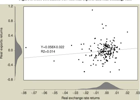
Figure 3 depicts a positive relationship between changes in real exchange rate and those of real exports in Egyptian case. This result means that excessive real exchange rate
volatility accentuate the real exports’ uncertainty, though this effect is weak.
With regard to our preliminary results, it is time to regress real exports returns on changes in real exchange rate.
4.2.Main findings: Estimates with energy versus without energy
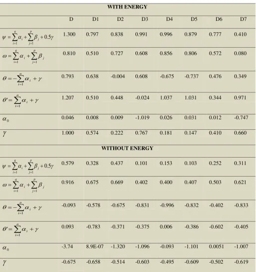
As we stated at the outset, we assess the linkage between real exchange rate returns and those of real exports using wavelet decomposition. We consider seven components or frequency bands, as we report in Table 4. This wavelet decomposition relies on a symmlet basis4.
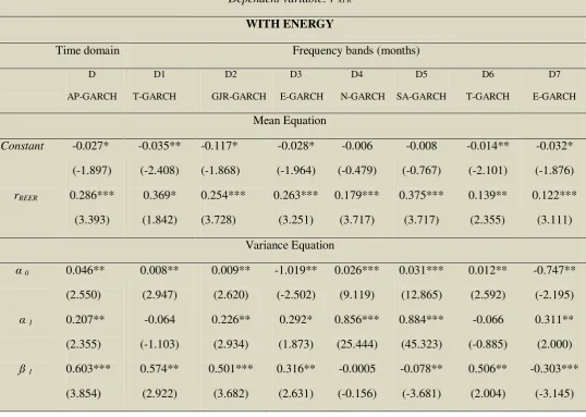
Our estimates of the optimal model chosen among various GARCH extensions under time domain and several frequency bands are summarized in Table 5. We find a significant and positive effect of real exchange rate returns on those of real exports (with energy) in Egyptian case, which is theoretically and empirically unexpected. However, studies on its fundamentals in developing countries emphasize that export performance-exchange rate uncertainty connection depends intensely to the volatile behavior of oil prices (e.g. Egert and
9
Zumaquero, 2007). Based on this assumption, we thought to subtract the share of oil from real exports and differential price. By doing so, we show a negative and significant linkage between the two variables, both in time domain and across the monthly frequencies.
4.2.1. Time domain
For the time domain, we observe in Table 5 that an increase in the real exchange rate by 10% prompts a significant increase in real exports by 2.86%. Contrary to expectations, we uncover a positive and significant correlation between our key variables for all returns from January 1994 to October 2009. This result changes substantively when subtracting the share of energy from total exports and differential price. Thus, we find that an appreciation of real exchange rate by 10% leads to a decrease in the level of real exports by 0.1%. This implies
that the energy’s share in total exports, which presents 26% (see Sekkat, 2012), makes a
difference in the considered relationship.
4.2.2. Frequency bands
For all considered frequencies (i.e. D1, D2, D3, D4, D5, D6 and D7), we find from Table 5 that the effect of real exchange rate returns on those of real exports is positive and significant. We observe that an increase in the real exchange rate by 10% yields an increase in real exports by 3.69%, 2.54%, 2.63%, 1.79%, 3.75%, 1.39% and 1.22%, respectively. This result is unexpected. The subtraction of energy leads to different results, which do not change substantively in terms of the sign from one frequency to another, whereas the magnitude of the effect depends to frequency transformations. Thus, an increase in the real effective exchange rate by 10% produces a drop in real exports by 0.05%, 0.13%, 0.01%, 0.02%, 0.18%, 0.23% and 0.19%, respectively during D1, D2, D3, D4, D5, D6 and D7. However, we
notice that at the lowest frequency, the coefficient associated to exchange rate uncertainty’s
effect on exports (with energy) is more intense than at the highest frequency and conversely for the case without energy.
10
is positive, which implies that the effect of bad news is more intense than that of good
news. In contrast, with subtracting energy, the coefficient is negative and significant, which
confirms asymmetry that is more vulnerable to good news than to bad news. As we depict in
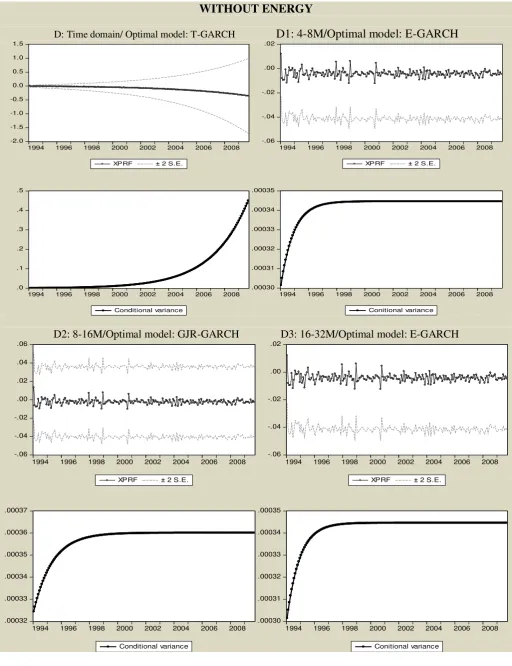
Figure 4, the conditional variance behaves better when we subtract energy’s share.
Without energy, this relationship behaves differently and therefore seems more intense at high time scale than at low frequency band. This result seems hardly surprising because of the important proportion of energy in the total of exports of Egypt (i.e. 26%). In addition, the real exchange rate is defined as the differential price of a basket of traded and non-traded goods between the domestic and the foreign economy leading to a great vulnerablity to the
volatility of commodity prices including those of oil. Previous studies highlight a complex
relationship between energy price and real exchange rate uncertainties, especially in oil exporting countries ; For example, Chen and Rogoff (2003), Engel and West (2005), Rogoff and Rossi (2010) and Bodenstein et al. (2011), among others.
4.3.Discussion of results
The varying results obtained with several time scales imply that the relationship between real exchange rate returns and changes in real exports is more complex than it may appear. Depending to frequency-to-frequency variation, it tends to be nonlinear and dependent on switching regimes (i.e. shifts and weights) or asymmetrical and dependent to leverage effects (i.e. good and bad news). As we depict in Table 4, the interaction between exchange volatility and exports (with energy) appears nonlinear at D, D2, D4 and D5 and asymmetrical under D1, D3, D6 and D7. Without energy, the link between both variables remain nonlinear in some frequencies and asymmetrical in other ones. At this stage, we can assert that the use of the best GARCH model among several GARCH extensions effectively differentiates all the
effects5. This can help the Egyptian authorities to better understand the evolution of exchange
rates and anticipate possible future shocks, including those related to changes in oil prices
5
11
In addition, for all studied cases (i.e. with and without energy and across different time scales), we note that the leverage effect impacts more the considered link than the switching regime. More precisely, we show that with energy the magnitude of exchange rate uncertainty’s effect on exports is equal to 2.61% (as average) when we account the sign of innovations comparable to 2.35% (as average) when we account structural breaks in the process of volatility. At the same way but less important, without energy, real exchange rate volatility’s effect on real exports is equal to 0.12% and 0.10%, respectively. Not surprisingly, in oil exporting economies that adopt managed exchange regime such as Egypt, the adjustment in real exchange rate will come through changes in consumer prices (e.g. Bouoiyour and Selmi, 2013). This implies that the differential price including that of oil price can make Egypt unable to adjust its currency and lead to excessive swings in real exchange
rates that affect intensely exports performance6.
With energy, the exchange uncertainty’s effect on real exports is greater at low
frequencies. This can be attributed mainly to speculative effects. More precisely, the energy market is a large market relative to other commodities and the assumption of financial
speculation may be evident.7 This leads to an increase of co movement between the spot price
of oil and futures prices. In related works, Alquist and Kilian (2010) and Fattouh et al. (2012) argue that the demand and supply shocks in the global oil market often entailed offsetting changes in oil inventories to reinforce then changes in oil prices, implying the presence of speculation. Furthermore, when the domestic country carries most of its trade with a single major country, pegging the local currency to the foreign one can mitigate exchange rate
uncertainty. However, the effective exchange rate can capture the value’s effects of the local
currency vis-à-vis the currencies of the trading partners (see Ngouana, 2012). Thus, Egyptian
trade may be affected by the euro’s movements, especially because its main exports partner is
Europe with share almost equal to 15.7% (see Appendix C). This implies also that the fluctuations of oil price denominated in dollar can coincide with a great volatility of euro. Accordingly, we depict in Appendix D that exports to European Union are dominated by
6
For details, we can refer to Sester (2007). This latter advance that “dollar pegs will not prevent the currencies of oil exporting economies from eventually appreciating in real terms.”
7For more details about how speculators can be drivers of oil price uncertainty, we can refer to Buyuksakin and
12
mineral and energy sectors, which are denominated on dollar and their prices are characterized by volatile behavior among all commodities in international market (e.g. Arezki et al. 2011).
Intuitively, because the differential price make a difference in the link in question, the above finding may be intensely due to the co-movement between energy price and the prices of other commodities (e.g. Baffes, 2007), especially because excessive speculation affects more oil markets. Speculation is also considered as a source of co-movement excess (e.g. Kratshell and Schmidt, 2012). Without energy, there is only co-movement between the prices of commodities (i.e. without including energy commodity price) which speculation is less important (e.g. Baffes, 2010). This can be the main reason behind the more intense exchange uncertainty’s effect on exports at high frequency band than low frequency.
Our results suggest that informations on respectively drivers and consequences of commodity prices’evolution including those of energy could be well recognised. Such information also about the exchange rate movements, the domestic and imported inflation rate and a clear understanding of the major channels through which oil price can affect real exchange rates and then real exports might be necessary. Egypt should improve coordination between monetary policy and fiscal policy to react quickly and effectively to external shocks..
5.
Conclusion
We have revisited the relationship between real exchange rate uncertainty and exports performance to check whether there is a significant short run dynamic between them. To do so, we combine wavelet analysis with an optimal model chosen among various GARCH
extensions (i.e. linear versus nonlinear, symmetrical versus asymmetrical, etc…).
The results reveal that the combination performed between wavelet decomposition and optimal GARCH model effectively enhance our understanding on the controversial link widely expected either theoretically or empirically. In this study, we show two main interesting results:
(i) With energy, real exports react more to real exchange rate volatility at low
13
(ii) Without energy, the relationship between exchange volatility and exports
performance behaves differently and therefore appears more intense at high time scale. This confirms the major role of speculation in energy market comparable to other commodities.
14
References
Achy, L. and Sekkat, K. (2003). “The European single currency and MENA‟s exports to
Europe.” Review of Development Economics 7, p. 563- 582.
Alquist R. and Kilian L. (2010). “What do we learn from the price of crude oil futures?”
Journal of Applied Econometrics 25, p. 539–573.
Arezki, R., Lederman, D. and Zhao, H. (2011). “The relative volatility of commodity prices: a
reappraisal.” IMF Working Papers 12/168, International Monetary Fund.
Anderson, T-G., Davis, R-A., Kreib, J-P. and Mikosh, T. (2009). Handbook of financial time
series. Springer publications.
Baffes, J. (2007). “Oil Spills on Other Commodities.” Resource Policy, 32(3), p.126-134.
Baffes, J. (2010). “More on the Energy/Non-Energy Commodity Price Link.” Applied
Economics Letters, 17(16), p. 1555-1558.
Bahmani-Oskooee, M. (2002). “Does Black Market Exchange Rate Volatility Deter the Trade
Flows? Iranian Experience.” Applied Economics, 34 (18), p. 2249-2255.
Benhmad, F. (2012). “Modeling nonlinear Granger causality between the oil price and US
dollar: A wavelet approach”. Economic modeling 29, p. 1505-1514.
Bera, A. K., and Higgins, M. L. (1993). “ARCH Models: Properties, Estimation and Testing,”
Journal of Economic Surveys, Vol. 7, No. 4, p. 307-366.
Bodenstein M., Erceg, C.J. and Guerrieri, L. (2011). “Oil shocks and external adjustment.”
Journal of International Economics, 83, p. 168-184.
Bollerslev, T. (1986). “Generalized autoregressive conditional heteroskedasticity.” Journal of
Econometrics, 31, p. 307-27.
Bollerslev, T., Engle, R.F and Nelson, D.B., (1993). “ARCH models” in Handbook of
Econometrics IV, Elsevier Science.
Bouoiyour J., Jellal M. and Selmi R., (2012). “Est-ce que les flux financiers réduisent la
15
Bouoiyour, J. and Selmi, R. (2013). “The controversial link between exchange rate volatility
and exports : Evidence from Tunisian case.” Economics Bulletin, Forthcoming.
Buyuksahin, B. and Harris J-H. (2011). “Do speculators drive crude oil futures prices?” The
Energy Journal, 32, p. 167–202.
Campbell, J. Y., Lo, A. W., and MacKinlay, A. C. (1997). “The Econometrics of Financial
Markets.” Princeton, New Jersey: Princeton University Press.
Chen, Y.-C. and Rogoff, K.S. (2003). “Commodity Currencies.” Journal of International
Economics, 60, p. 133-160.
Ćorić, B. and Pugh, G. (2010). “The effects of exchange rate variability on international
trade: a metaregression analysis.” Applied Economics, 42, p. 2631-2644.
Ding Z., Granger, C.W. and Engle, R.F., (1993). “A long memory property of stock market
returns and a new model.” Journal of Empirical Finance 1, p. 83-106.
Duan, J. (1997). “Augmented GARCH(p,q) process and its diffusion limit.” Journal of
Econometrics 79(1), p. 97–127.
Engel, C.N.M. and West, K.D. (2005). “Exchange rates and fundamentals.” Journal of
Political Economy 113, p.485-517.
Engle, R.F. (1982). “Autoregressive Conditional Heteroskedasticity with Estimates of U.K.
inflation.” Econometrica, 50, p. 987-1008.
Engle, R. F., Lilien, D. M. and Robins, R. P., (1987). “Estimating Time Varying Risk Premia
in the Term Structure: The ARCH-M Model.” Econometrica 55, p. 391-407.
Égert, B. and Morales-Zumaquero, A. (2007). “Exchange Rate Regimes, Foreign Exchange
Volatility and Export Performance in Central and Eastern Europe: Just Another Blur
Project?” William Davidson Institute Working Papers Series wp782.
Epinoza, R. and Prasad, A. (2012). “Monetary policy transmission in the GCC countries”
16
Fattouh, B., Kilian, L. and Mahadeva, L. (2012). “The role of speculation in oil markets:
What have we learned so far?” CEPR Discussion Paper DP8916, Center for Economic
Policy Research.
Gosten, L. R., Jagannathan, R. and Runkle, D. E. (1993). “On the relation between the
expected value and the volatility of the nominal excess return on stocks”. The Journal of Finance 48 (5), p.1779-1801
Gourinchas, P.O. and Rey, H. (2007). “International financial adjustment.” Journal of
political economy, 115 (4), p. 665-703.
Granger, C.W.J., Ding, Z. and Engle R.F. (1993). “A Long Memory Property of Stock Market Returns and a New Model.” Journal of Empirical Finance 1, p. 83–106.
Haile Gebretsadik, M. and Pugh, G. (2011). “Does exchange rate volatility discourage
international trade? A meta-regression analysis.” The Journal of International Trade
and Economic Development, DOI:10.1080/09638199.2011.565421
Hansen, P.R. (2001). “A test for superior predictive ability.” Brown University, Department
of Economics Working Paper 2001–06 (http://www.econ.brown.edu/fac/Peter Hansen).
Higgins, M.L. and Bera, A.K. (1992). “A Class of nonlinear ARCH models”. International
Economic Review 33, p. 137-58.
Kandil, M. and Dincer Nergiz, N. (2008). “A comparative analysis of exchange rate
fluctuations and economic activity: The cases of Egypt and Turkey”. International
Journal of Development Issues, Emerald Group Publishing 7, p. 136-159.
Kamar, B. (2004). “De facto exchange rate policies in the MENA region: Toward deeper
cooperation.” Economic Research Forum for the Arab countries, Beirut, Lebanon.
Kim, S. and In, H.F., (2003). “The relationship between financial variables and real
economic activity: evidence from spectral and wavelet analyses.” Studies in Nonlinear Dynamics and Econometrics 7, Article 4.
Kratschell, K. and Schmidt, T. (2012). “Long-run trends or short-run fluctuations: what
17
Maheu, J.M. and McCurdy, T.H. (2004). “News arrival, jump dynamics, and volatility components for individual stock returns.” Journal of Finance 59(2).
Mazur, B. and Pipien, M. (2012). “On the empirical importance of periodicity in the volatility
of financial time series.” National Bank of Poland Working Papers 124, National Bank
of Poland, Economic Institute.
McKenzie, D., (1998).“The Impact of Exchange Rate Volatility on Australian Trade Flows.”
Journal of International Financial Markets.” Institutions and Money 8, p.21- 38.
Nabli M-K., Keller J. and Véganzonès-Varoudakis M. (2004). “Exchange Rate Management
within the Middle East and North Africa Region: the Cost to Manufacturing
Competitiveness.” Working paper n° 81, American University of Beirut, p.1-23.
Nelson D-B., (1991). “Conditional heteroskedasticity in asset returns: A new approach.”
Econometrica 59, p. 347-370.
Sekkat, K. (2012). “Manufactured exports and FDI in Southern Mediterranean countries :
Evolution, determinants and prospects,” MEDPRO Technical report n°14.
Sester, B. (2007). “The case for exchange rate flexibility in oil exporting economies.”
Peterson Institute for International Economics, working paper n° PB0708.
Tong H., (1990). “Nonlinear time series analysis since 1990: Some personal reflections.”
University of Hong Kong and London school economics.
Vergil, H., (2002). “Exchange rate volatility in Turkey and its effects on trade flows.” Journal of Economic and Social Research 4 (1), p. 83-99.
Zakoian, J-M. (1994). “Threshold Heteroskedastic Models.” Journal of Economic Dynamics
and Control 18, p. 931-5.
18
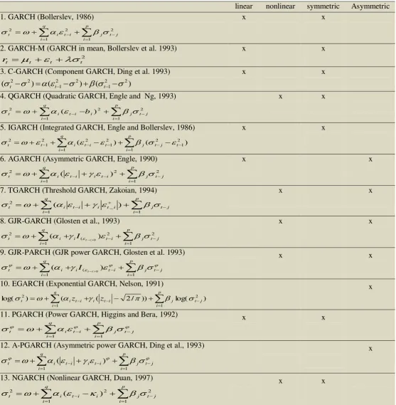
Table 1. GARCH extensions
linear nonlinear symmetric Asymmetric 1. GARCH (Bollerslev, 1986)
p i j t j q i i t i t 1 2 1 22
x x
2. GARCH-M (GARCH in mean, Bollerslev et al. 1993) 2
t t
t t
r
x x
3. C-GARCH (Component GARCH, Ding et al. 1993) )
( ) (
)
( 2 2
1 2
2 1 2
2
t t t
x x
4. QGARCH (Quadratic GARCH, Engle and Ng, 1993)
p i j t j i q i i t i t b 1 2 2 12 ( )
x x
5. IGARCH (Integrated GARCH, Engle and Bollerslev, 1986)
) ( ) ( 1 2 1 2 1 2 1 2 2 1
2
p i t j t j q i t i t i t
t
x x
6. AGARCH (Asymmetric GARCH, Engle, 1990)
p i j t j q i i t i i t i t 1 2 2 12 ( )
x x
7. TGARCH (Threshold GARCH, Zakoian, 1994)
p i j t j q i i t i i t i t 1 1 _ 2 ) ( x x
8. GJR-GARCH (Glosten et al., 1993)
p
i j t j i t i q i i
t I t i
1 2 2
( 1
2 ( )
0
x x
9. GJR-PARCH (GJR power GARCH, Glosten et al. 1993)
p
i j t j i t i q i i
t I t i
1 (
1
)
( 0
x x
10. EGARCH (Exponential GARCH, Nelson, 1991)
p i j t j i t i q i i t it z z
1
2 1
2) ( ( 2/ )) log( )
log(
x
11. PGARCH (Power GARCH, Higgins and Bera, 1992)
p i j t j i t q i i t 1 1 x x
12. A-PGARCH (Asymmetric power GARCH, Ding et al., 1993)
p i j t j q i i t i i t i t 1 1 ) ( x13. NGARCH (Nonlinear GARCH, Duan, 1997)
p i j t j q i i i t i t 1 2 1 22 ( )
x x
Notes: 2
t
: conditional variance, t: conditional standard deviation, : reaction of shock, 0: reaction of shock, 1:
ARCH term,1: GARCH term, : error term; It: denotes the information set available at time t; It-1: denotes the information set
available at time t-1;zt : the standardized value of error term where zt t1/t1; : innovation, : leverage
19
Figure 1. Real exports and real effective exchange rate (Normalized data)
Source: IMF, IFS and EconstatsTM.
Figure 2. Real exports and real exchange rate returns (Normalized data)
Source: IMF, IFS and EconstatsTM and authors’calculations. -4
-3 -2 -1 0 1 2 3
94 95 96 97 98 99 00 01 02 03 04 05 06 07 08 09
Real exports (log)
Real effective exchange rate (log)
-8 -6 -4 -2 0 2 4 6
94 95 96 97 98 99 00 01 02 03 04 05 06 07 08 09
[image:20.595.77.526.398.656.2]20
Table 2. Criteria used on the choice of the optimal GARCH model
Akaike criterion : -2log(vraisemblance)+2k
Bayesian criterion : -2log(vraisemblance)+log(N).k
Hannan-Quinn criterion : -2log(vraisemblance)+2k.log(log(N))
[image:21.595.43.554.259.322.2]Note: k the degree of freedom and N the number of observations.
Table 3. Descriptive statistics
Mean Median Maximum Minimum Std. Dev. Skewness Kurtosis J-Bera
rXPR -0.0098 -0.0165 1.105350 -0.58324 0.213640 0.836873 7.647297 192.1405
rREER -0.0022 -0.0005 0.020377 -0.07770 0.010460 2.85336 18.53189 2156.226
[image:21.595.74.522.381.701.2]Note: rXPR : Real exports returns ; rREER : Real exchange rate returns.
Figure 3. First correlation between real exports and real exchange rate
-0.8 -0.4 0.0 0.4 0.8 1.2
R
e
a
l
e
x
p
o
rt
s
r
e
tu
rn
s
-.08 -.07 -.06 -.05 -.04 -.03 -.02 -.01 .00 .01 .02 .03
Real exchange rate returns Y=0.058X-0.022
21
Table 4. Frequency bands
Scales Monthly frequencies
D1 2-4
D2 4-8
D3 8-16
D4 16-32
D5 32-64
D6 64-128
D7 >128
Table 5. The link between changes in real exchange rate and those of real exports: Parameters of optimal GARCH model
Dependent variable: r XPR
WITH ENERGY
Time domain Frequency bands (months)
D AP-GARCH D1 T-GARCH D2 GJR-GARCH D3 E-GARCH D4 N-GARCH D5 SA-GARCH D6 T-GARCH D7 E-GARCH Mean Equation Constant rREER -0.027* (-1.897) 0.286*** (3.393) -0.035** (-2.408) 0.369* (1.842) -0.117* (-1.868) 0.254*** (3.728) -0.028* (-1.964) 0.263*** (3.251) -0.006 (-0.479) 0.179*** (3.717) -0.008 (-0.767) 0.375*** (3.717) -0.014** (-2.101) 0.139** (2.355) -0.032* (-1.876) 0.122*** (3.111) Variance Equation
α 0
α 1
ß 1
[image:22.595.31.570.374.757.2]22
Y 1.000*
(1.698) 0.574*** (4.820) 0.222** (2.934) 0.767*** (8.250) 0.181 (0.459) 0.147** (2.398) 0.410*** (3.617) 0.660*** (3.441) WITHOUT ENERGY
Time domain Frequency bands (months)
D T-GARCH D1 E-GARCH D2 GJR-GARCH D3 E-GARCH D4 T-GARCH D5 N-GARCH D6 SA-GARCH D7 E-GARCH Mean Equation Constant rREER -0.0003 (-0.579) -0.010** (-2.913) -0.001*** (-5.800) -0.005** (-2.423) -0.018* (-1.641) -0.013*** (-4.259) -0.0005* (-1.819) -0.001* (-1.597) -0.0011 (-0.459) -0.002** (-2.315) -0.007* (-1.728) -0.018* (-1.496) -0.0002 (-0.891) -0.023** (-2.119) -0.016* (-1.637) -0.019** (-2.085) Variance Equation
α 0
α 1
ß 1
Y -3.74*** (-4.833) 0.768*** (5.372) 0.148* (1.615) -0.675** (-2.926) 8.9E-07** (2.720) -0.098*** (-6.359) 0.755*** (4.622) -0.658*** (-4.101) -1.320** (-2.099) 0.143* (1.781) 0.526*** (9.703) -0.514** (-2.832) -1.096** (-2.105) 0.228** (2.000) 0.174* (1.918) -0.603* (-1.609) -0.093 (-1.303) 0.501* (1.810) -0.101** (-2.054) -0.495** (-2.223) -1.101 (-0.766) 0.223*** (4.664) 0.184** (2.930) -0.609** (-2.415) 0.0051* (1.699) -0.10*** (-3.254) 0.513* (1.708) -0.502* (-1.688) -1.007 (-0.832) 0.214* (1.653) 0.407** (2.133) -0.619** (-2.115)
Note: standard deviations are in parentheses, *** significant at 1%, ** 5% * 10%. r XPR : changes in oil prices; r REER: changes in real
23
Table 6. Persistence of conditional variance
WITH ENERGY
D D1 D2 D3 D4 D5 D6 D7
0.5
1 1
q i p j j i1.300 0.797 0.838 0.991 0.996 0.879 0.777 0.410
q i p j j i 1 1 0.810 0.510 0.727 0.608 0.856 0.806 0.572 0.080
a i i 10.793 0.638 -0.004 0.608 -0.675 -0.737 0.476 0.349
a i i 1' 1.207 0.510 0.448 -0.024 1.037 1.031 0.344 0.971
0
0.046 0.008 0.009 -1.019 0.026 0.031 0.012 -0.747
1.000 0.574 0.222 0.767 0.181 0.147 0.410 0.660WITHOUT ENERGY
0.5
1 1
q i p j j i0.579 0.328 0.437 0.101 0.153 0.103 0.252 0.311
q i p j j i 1 1 0.916 0.675 0.669 0.402 0.400 0.407 0.503 0.621
a i i 1-0.093 -0.578 -0.675 -0.831 -0.996 -0.832 -0.402 -0.833
a i i 1' 0.093 -0.783 -0.371 -0.375 0.006 -0.386 -0.602 -0.405
0
-3.74 8.9E-07 -1.320 -1.096 -0.093 -1.101 0.0051 -1.007
-0.675 -0.658 -0.514 -0.603 -0.495 -0.609 -0.502 -0.61924
Figure 4. Conditional variance under Time domain and frequency bands by using optimal GARCH model
WITHOUT ENERGY
D: Time domain/ Optimal model: T-GARCH D1: 4-8M/Optimal model: E-GARCH
D2: 8-16M/Optimal model: GJR-GARCH D3: 16-32M/Optimal model: E-GARCH
-2.0 -1.5 -1.0 -0.5 0.0 0.5 1.0 1.5
1994 1996 1998 2000 2002 2004 2006 2008
XPRF ± 2 S.E.
.0 .1 .2 .3 .4 .5
1994 1996 1998 2000 2002 2004 2006 2008
Conditional variance
-.06 -.04 -.02 .00 .02
1994 1996 1998 2000 2002 2004 2006 2008
XPRF ± 2 S.E.
.00030 .00031 .00032 .00033 .00034 .00035
1994 1996 1998 2000 2002 2004 2006 2008
Conitional variance
-.06 -.04 -.02 .00 .02 .04 .06
1994 1996 1998 2000 2002 2004 2006 2008
XPRF ± 2 S.E.
.00032 .00033 .00034 .00035 .00036 .00037
1994 1996 1998 2000 2002 2004 2006 2008
Conditional variance
-.06 -.04 -.02 .00 .02
1994 1996 1998 2000 2002 2004 2006 2008
XPRF ± 2 S.E.
.00030 .00031 .00032 .00033 .00034 .00035
1994 1996 1998 2000 2002 2004 2006 2008
25 D4: 32-64M/Optimal model: T-GARCH D5: 64-128M/ Optimal model: N-GARCH
-.06 -.04 -.02 .00 .02 .04 .06
1994 1996 1998 2000 2002 2004 2006 2008
XPRF ± 2 S.E.
.00032 .00033 .00034 .00035 .00036 .00037
1994 1996 1998 2000 2002 2004 2006 2008
Conditional variance
-2.0 -1.5 -1.0 -0.5 0.0 0.5 1.0 1.5
1994 1996 1998 2000 2002 2004 2006 2008
XPRF ± 2 S.E.
.0 .1 .2 .3 .4 .5
1994 1996 1998 2000 2002 2004 2006 2008
Conditional variance
-.04 -.02 .00 .02 .04
1994 1996 1998 2000 2002 2004 2006 2008 XPRF ± 2 S.E.
.00000 .00004 .00008 .00012 .00016 .00020
1994 1996 1998 2000 2002 2004 2006 2008 Conditional variance
-.06 -.04 -.02 .00 .02 .04 .06
1994 1996 1998 2000 2002 2004 2006 2008 XPRF ± 2 S.E.
.00032 .00033 .00034 .00035 .00036 .00037
26 D6: 64-128M/ Optimal model: SA-GARCH D7: >128M/ Optimal model: E-GARCH
WITHOUT ENERGY
D: Time domain/ Optimal model: AP-GARCH D1: 4-8M/Optimal model: T-GARCH
-2.0 -1.5 -1.0 -0.5 0.0 0.5 1.0 1.5
1994 1996 1998 2000 2002 2004 2006 2008
XPRF ± 2 S.E.
.0 .1 .2 .3 .4 .5
1994 1996 1998 2000 2002 2004 2006 2008
Conditional variance
-.06 -.04 -.02 .00 .02
1994 1996 1998 2000 2002 2004 2006 2008
XPRF ± 2 S.E.
.00030 .00031 .00032 .00033 .00034 .00035
1994 1996 1998 2000 2002 2004 2006 2008
Conitional variance
-1.5 -1.0 -0.5 0.0 0.5 1.0 1.5
1994 1996 1998 2000 2002 2004 2006 2008
XPRF ± 2 S.E.
.00 .05 .10 .15 .20 .25 .30 .35
1994 1996 1998 2000 2002 2004 2006 2008
Conditional variance
-1.5 -1.0 -0.5 0.0 0.5 1.0 1.5
1994 1996 1998 2000 2002 2004 2006 2008
XPRF ± 2 S.E.
.0 .1 .2 .3 .4 .5
1994 1996 1998 2000 2002 2004 2006 2008
27 D2: 8-16M/Optimal model: GJR-GARCH D3: 16-32M/Optimal model: W-GARCH
D4: 32-64M/Optimal model: W-GARCH D5: 64-128M/ Optimal model: SA-GARCH
-1.5 -1.0 -0.5 0.0 0.5 1.0 1.5
1994 1996 1998 2000 2002 2004 2006 2008
XPRF ± 2 S.E.
.0 .1 .2 .3 .4
1994 1996 1998 2000 2002 2004 2006 2008
Conditional variance
-1.0 -0.5 0.0 0.5 1.0 1.5 2.0
1994 1996 1998 2000 2002 2004 2006 2008
XPRF ± 2 S.E.
.329 .330 .331 .332 .333 .334 .335
1994 1996 1998 2000 2002 2004 2006 2008
Conditional variance
-1.6 -1.2 -0.8 -0.4 0.0 0.4
1994 1996 1998 2000 2002 2004 2006 2008 XPRF ± 2 S.E.
.0 .1 .2 .3 .4 .5
1994 1996 1998 2000 2002 2004 2006 2008 Conditional variance
-1.5 -1.0 -0.5 0.0 0.5 1.0 1.5
1994 1996 1998 2000 2002 2004 2006 2008 XPRF ± 2 S.E.
.0 .1 .2 .3 .4
28 D6: 64-128M/ Optimal model: TGARCH D7: >128M/ Optimal model: E-GARCH
Note: Own calculation.
-1.5 -1.0 -0.5 0.0 0.5 1.0 1.5
1994 1996 1998 2000 2002 2004 2006 2008 XPRF ± 2 S.E.
.0 .1 .2 .3 .4 .5
1994 1996 1998 2000 2002 2004 2006 2008 Conditional variance
-1.6 -1.2 -0.8 -0.4 0.0 0.4
1994 1996 1998 2000 2002 2004 2006 2008 XPRF ± 2 S.E.
.0 .1 .2 .3 .4 .5
29
Appendices
Appendix A. Wavelets of real exports and real exchange rate returns (WITH ENERGY) -20 -10 0 10 20 30 40
1994 1996 1998 2000 2002 2004 2006 2008
D1 -1.2 -0.8 -0.4 0.0 0.4 0.8
1994 1996 1998 2000 2002 2004 2006 2008
D2 -50 0 50 100 150 200 250
1994 1996 1998 2000 2002 2004 2006 2008
D3 -8 -4 0 4 8 12 16 20 24
1994 1996 1998 2000 2002 2004 2006 2008
D4 -20 -10 0 10 20
1994 1996 1998 2000 2002 2004 2006 2008
D5 -8 -4 0 4 8
1994 1996 1998 2000 2002 2004 2006 2008
D6 -6 -4 -2 0 2 4 6 8
1994 1996 1998 2000 2002 2004 2006 2008
D7
Wav elet decomposition of real exports returns
-4 -2 0 2 4 6 8 10
1994 1996 1998 2000 2002 2004 2006 2008
D1 -20 0 20 40 60 80
1994 1996 1998 2000 2002 2004 2006 2008
D2 -1.00 -0.75 -0.50 -0.25 0.00 0.25 0.50
1994 1996 1998 2000 2002 2004 2006 2008
D3 -5 0 5 10 15 20 25
1994 1996 1998 2000 2002 2004 2006 2008
D4 -10 -5 0 5 10 15 20 25
1994 1996 1998 2000 2002 2004 2006 2008
D5 -8 -4 0 4 8 12
1994 1996 1998 2000 2002 2004 2006 2008
D6 -100 -80 -60 -40 -20 0 20
1994 1996 1998 2000 2002 2004 2006 2008
D7
30
Appendix B. Wavelets of real exports and real exchange rate returns (WITHOUT ENERGY) -4 -2 0 2 4 6
1994 1996 1998 2000 2002 2004 2006 2008
D1 -30 -20 -10 0 10 20 30 40
1994 1996 1998 2000 2002 2004 2006 2008
D2 -1.00 -0.75 -0.50 -0.25 0.00 0.25 0.50
1994 1996 1998 2000 2002 2004 2006 2008
D3 -100 0 100 200 300 400 500
1994 1996 1998 2000 2002 2004 2006 2008
D4 -10 0 10 20 30
1994 1996 1998 2000 2002 2004 2006 2008
D5 -1 0 1 2 3
1994 1996 1998 2000 2002 2004 2006 2008
D6 -4 0 4 8 12
1994 1996 1998 2000 2002 2004 2006 2008
D7
Wav elet decomposition of real exports returns
-100 -80 -60 -40 -20 0 20
1994 1996 1998 2000 2002 2004 2006 2008
D1 -800 -600 -400 -200 0 200
1994 1996 1998 2000 2002 2004 2006 2008
D2 -1.00 -0.75 -0.50 -0.25 0.00 0.25 0.50
1994 1996 1998 2000 2002 2004 2006 2008
D3 -4,000 -3,000 -2,000 -1,000 0 1,000
1994 1996 1998 2000 2002 2004 2006 2008
D4 -10 -5 0 5 10 15 20
1994 1996 1998 2000 2002 2004 2006 2008
D5 -3,000 -2,500 -2,000 -1,500 -1,000 -500 0 500
1994 1996 1998 2000 2002 2004 2006 2008
D6 -400 -300 -200 -100 0 100
1994 1996 1998 2000 2002 2004 2006 2008
D7
31
Appendix C. Egyptian main trade partners
Note: For more details, see this link: http://trade.ec.europa.eu/doclib/docs/2006/september/tradoc_113375.pdf
Appendix D. Egyptian exports composition (to Europe)
Note: For more details, see this link: http://trade.ec.europa.eu/doclib/docs/2006/september/tradoc_113375.pdf 14,80% 5,40%
4,60% 2,40%
2,20% 2,10% 1,90% 1,80% 1,50% 1,40%
0,00% 2,00% 4,00% 6,00% 8,00% 10,00% 12,00% 14,00% 16,00%
EU27 USA China Kuwait Turkey Saudi Arabia Russia Brazil Ukraine South Korea
Mineral products (inUS $)
16%
Chemical products (in $) 17%
Oil crude (in $) 9% manufactured
products and foods (in euro) 58% (including