Urban Density and Climate Change: A STIRPAT Analysis using City level Data

(1)

Urban Density and Climate Change: A

STIRPAT Analysis using City-level Data

Liddle, Brantley

2013

Online at

https://mpra.ub.uni-muenchen.de/52089/

(2)

Brantley Liddle

Senior Research Fellow

Centre for Strategic Economic Studies Victoria University

Level 13, 300 Flinders Street Melbourne, VIC 8001 Australia

btliddle@alum.mit.edu

ABSTRACT

Two important, increasing trends for those concerned about climate change to consider are urbanization/the importance of cities and energy used in transport—particularly energy used to achieve personal mobility. While national urbanization levels are not a good indicator of urban transport demand, there is an established negative relationship between urban density and such demand. This paper uses a consistent, well-known population-based framework (the STIRPAT model) and three separate, but highly related, datasets of cities from developed and developing countries (with observations from 1990, 1995, and 2001) to examine the relationship among private transport energy consumption, population, income, urban density, and several variables (e.g., network size and prices) that describe the nature of the public and private transport systems of those cities. The paper confirms the now well-established result that urban density is

negatively correlated with urban private transport energy consumption. In terms of policies, improving private vehicle fuel efficiency, in particular, and increasing fuel price as well as other ownership/operating costs for private transport could have a substantial impact on lowering transport energy consumption. On the other hand, there is no evidence that further lowering the cost to riders of public transport would lower private transport energy consumption. For cities in developing countries, demographic variables (population size and urban density) are particularly important in determining private transport energy consumption. Also, private transport energy consumption is considerably less price sensitive in those developing country cities compared to cities in the most developed countries.

Keywords: urban density; STIRPAT; transport energy demand; city-based data.

(3)

1. Introduction and background

The level of world urbanization crossed the 50% mark in 2009; the United Nations

expects that over the next 40 years, urban areas will absorb all of the projected 2.3 billion global

population growth while urban areas will continue to draw in some rural population. In addition,

most of the population growth expected in urban areas will be concentrated in less developed

regions. At the same time, transport contributes more than one-fifth of global anthropogenic

carbon dioxide emissions; furthermore, transport energy consumption is increasing in both

developed and developing countries and is a carbon-intensive activity everywhere. To illustrate,

for International Energy Agency (IEA) countries as a whole, carbon emissions from

manufacturing industries and construction and from the residential sector (i.e., housing) both

declined by around 20% from 1971-2007, but emissions from road transport more than doubled

over that period (data from IEA).

While national urbanization levels are not a particularly good indicator of transport

demand (Liddle and Lung 2010), several studies have shown a (negative) relationship between

urban density and vehicle miles traveled or energy consumed in private transport, using

city-based data (e.g., Newman and Kenworthy 1989; Kenworthy and Laube 1999; Romero-Lankao et

al. 2009; Karathodorou et al. 2010; and Travisi et al. 2010). This paper uses the well-known

STIRPAT model and three separate, but highly related, datasets of cities from developed and

developing countries to examine the relationship among (aggregate) private transport energy

consumption, population, income, urban density, and several variables (e.g., network size and

prices) that describe the nature of the public and private transport systems of those cities. In

doing so, the paper is similar to Romero-Lankao et al. (2009), but expands on that work by

(4)

know of that considers all three of these related datasets), and by considering additional

explanatory variables (largely taken from economics) that also can be considered policy

variables.

A popular framework used to distinguish between population’s and GDP’s (or income’s)

impact on the environment is Dietz and Rosa’s (1997) STIRPAT (Stochastic Impacts by

Regression on Population, Affluence, and Technology). STIRPAT builds on IPAT/impact

equation of Ehrlich and Holdren (1971):

T A P

I = × × (1)

Where I is environmental impact, P is population, A is affluence or consumption per capita, and

T is technology or impact per unit of consumption. Dietz and Rosa (1997) addressed the criticism

that the Ehrlich-Holdren/IPAT framework does not allow hypothesis testing by proposing a

stochastic version of IPAT:

(2)

i d i c i b

i A T e

aP I =

Where the subscript i denotes cross-sectional units (e.g., countries), the constant a and exponents

b, c, and d are to be estimated, and e is the residual error term.

Since Equation 2 is linear in log form, the estimated exponents can be thought of as

elasticities (i.e., they reflect how much a percentage change in an independent variable causes a

percentage change in the dependent variable). In addition to determining whether population or

GDP has a greater marginal impact on the environment, another important/popular hypothesis to

test is whether population’s elasticity is different from unity. That hypothesis is worth testing

(5)

variable via division (in Equation 2), and so the dependent variable would be in per capita terms

as is often the case in non-STIRPAT analyses (like those in the so-called Environmental Kuznets

Curve or EKC literature). Also, the T term can now be treated more like an intensity of use

variable and be modelled as a combination of log-linear factors.

2. Data and models

The STIRPAT model typically is employed with national level data. There are a few

single-country studies using local level data, typically the US and typically county level (e.g.,

DeHart and Soule 2000; Squalli 2009; and Roberts 2011); the only other STIRPAT study we

know of to use both city-based data and locally-based, cross-national data is Romero-Lankao et

al. (2009).

The first of the three transport and cities datasets used here is Kenworthy et al. (1999). It

contains data from 1960, 1970, 1980, and 1990, but economic data (GDP per capita and

prices/costs) is available only for 1990. Cities from Asia, Australia, Europe, and North America

(46 in total) are included (the specific cities used here from each of the three datasets are

displayed in Appendix Table A-1). The Millennium Cities Database for Sustainable Transport

(Kenworthy and Laube 2001) is by far the largest of the three, both in terms of the indicators

collected and the cities covered. It contains 1995 data for 100 cities (which comprised a total

population of over 400 million in 1995)—included is nearly every city with more than 2 million

inhabitants that is located in an International Union for Public Transport (UITP) member

country. There also are a substantial number of cities from developing countries, including ones

from Africa, Middle East, and South America. Lastly, the Mobility in Cities Database (UITP

2005) contains 2001 data for 50 cities. The UITP aimed to have the Kenworthy and Laube

(6)

contained in UITP (2005), and some of the remaining indicators have slightly changed

definitions. Furthermore, nearly all of the cities in UITP (2005) are European.

By far the most popularly used datasets are the ones drawing on the 1990 and 1995 data

(Romero-Lankao et al. 2009 employ Kenworthy and Laube 2001). Indeed, we know of only one

published paper that depends on UITP (2005).1

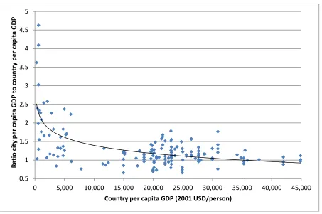
Because of indicator availability, this study uses data from 167 cities (from 1990, 1995,

and 2001). In Figure 1, the ratio of city GDP per capita to the associated country GDP per capita

is plotted against that country GDP per capita for 160 of those cities.2 There are two interesting

observations. First, most of the cities have higher GDP per capita than their respective countries

as a whole—the ratio of GDPs is below one for only 35 cities, and below 0.85 for only 14.

Second, the relative economic importance of cities is stronger in countries with lower GDP per

capita. That second point demonstrates the important migratory pull cities have in developing

countries, and provides insight into why the vast majority (20 of 26) of megacities (cities with

populations over 10 million) are located in less developed countries, and why the UN projects all

future population growth (over the next 40 years) will be located in urban areas.

Figure 1

2.1 Variables analyzed

As a dependent variable, we focus on (aggregate) private transport energy consumption

(measured in megajoules3) as opposed to total energy consumption (the dependent variable

considered in Romero-Lankao et al. 2009); we do so because public transport is the main

mobility alternative to private transport, and we aim, in part, to explain this choice. Since private

1

That paper, Albalate and Bel (2010), focuses on public transit provision in Europe.

2

The city-states Hong Kong and Singapore and Taipei, Taiwan have been excluded from this figure, and from all other city-to-nation comparisons.

3

(7)

transport is much more energy intensive than public transport, a major way cities can lower their

transport energy consumption is to shift mobility away from private to public modes. Indeed, for

the cities studied here, the average ratio of private to public transport intensity (energy consumed

divided by passenger kilometers driven/provided) is 4.4, and in all but 10 cities, private transport

was at least 50% more energy intensive (the ratio was below one only for Glasgow in 1995).

In addition to GDP per capita and total population, we consider several intensity variables

(the “T-type” variables from Equation 2). The main intensity variable used here is urban

density—indeed, urban density is a primary motivation for the use of these datasets by all

researchers. As mentioned above, the negative correlation between private transport use and

urban density was established by Newman and Kenworthy (1989) and has been confirmed by

several studies since then. Although there is still debate about the causal mechanism involved,

we agree with Rickwood et al. (2008) that the most compelling explanation is that “… there is a

positive feedback loop between transport and land use such that public transport friendly land

use encourages less automobile travel and more public transport travel, which in turn encourages

public transport friendly land use…” (Rickwood et al. 2008, p. 74).

The relationship between urban density of cities and some related national-level

indicators may be surprising. For the sample used here, the correlation (ρ) between urban density

and the corresponding national population density is only 0.35, and national urbanization levels

are actually negatively correlated with urban density (ρ = -0.59). Figure 2 shows, for the data

used here, the relationship between urban private transport energy use per capita (the dependent

variable) and both urban density (the upper graph) and the corresponding national urbanization

level (the lower graph). The upper graph displays the now well-known negative, nonlinear

(8)

1989; Kenworthy and Laube 1999); whereas, the bottom graph shows the weaker and, perhaps

surprising, positive relationship between urban private transport and urbanization level. That

higher levels of national urbanization are correlated with greater levels of urban private transport

most likely reflects the positive correlation between urbanization and income (ρ = 0.61 for the

countries represented in this study).

Figure 2

In their analysis of total energy from transport, Romero-Lankao et al. (2009) considered

the percentage of public transportation use in cities. Rather than use that variable, we use a series

of variables designed to infer the private vs. public transport choice. The first of those variables

involves the costs of private and public transport: fuel price, the cost per passenger kilometer of

private transport (which, in addition to fuel, includes maintenance, insurance, and taxes, among

other costs), and the cost to the traveler of one public transport kilometer. As well as representing

the economic choice facing city inhabitants, differences in these prices across cities represent the

broader society values of public and private transport. One would expect higher fuel and private

per kilometer costs to discourage private transport and thus lower private transport energy

consumption; whereas, higher public per kilometer costs would discourage public transport and

thus raise private energy consumption. The other choice-based variable relates to the public

transport network coverage: the public transport seat kilometers of service offered per city

inhabitant. The larger that indicator, the better the public transport alternative would be for

achieving desired mobility, and thus, the lower private transport energy consumption should be.

The last independent variable considered is fuel efficiency. Fuel efficiency is clearly the

key factor in the relationship between vehicle miles traveled (VMT) and transport fuel

(9)

influenced by fuel price (e.g., Karathodorou et al. 2010). We include both fuel price and fuel

efficiency for several reasons.

First, the fuel price indicator is only available for the 1995 dataset, whereas fuel

efficiency can be estimated for all three datasets. Second, the measure of fuel efficiency used is

based on travel and energy consumption within the urban borders averaged across several

vehicle modes (passenger cars, motorcycles, and taxis). Thus, the measure of effective fuel

efficiency for private urban travel may differ from the overall fuel efficiency of a country’s

vehicle fleet, and it is that second measure of efficiency that is most likely to have a strong

association to fuel price. Indeed, the correlation between the fuel efficiency and fuel price

measures used here is only 0.22.

Lastly, fuel efficiency, like many of the independent variables, can be thought of as a

policy variable/lever that can be adjusted via national vehicle fuel efficiency standards. Fuel

price, of course, can be and is affected by taxes. The cost of private transport travel can be

further affected by vehicle registration, parking, and road-use tolls; whereas, public transport can

be encouraged by ticket subsidies and/or frequent traveler discounts and investment in network

coverage. Urban density also can be influenced through various policies, but probably less

directly and arguably less effectively so than the previous variables. Table 1 lists the variables

used, their definitions and units, and their coverage in the three datasets.

Table 1

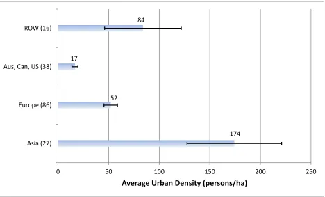
We do not consider any geography-based dummy variables, in part, because the urban

density variable appears to play that role very well. Figure 3 displays the average urban density

(10)

rest of world group. Figure 3 also shows the 99% confidence bounds for those averages (the

error bars).

Figure 3

Not surprisingly, Australian, Canadian, and US cities have by far the lowest average

urban density—the very cities for which Newman and Kenworthy (1989) coined the term

dependent. European cities have average urban densities considerably higher than those

auto-dependent cities, and Asian cities have average urban densities considerably higher than the

European ones. Also, for those three groups, their averages are all highly significantly different

from one another. The rest of world cities (mostly drawn from developing countries) have an

average urban density between Europe’s and Asia’s. However, that average is not statistically

different from Europe’s (not very surprising given the diversity in the rest of world group).

Table 2 displays some descriptive statistics (means and standard deviations) for each of

the variables considered and for each dataset used. Table 2 also splits the 1995 dataset into cities

from developed and from less developed countries for reasons that will be made clear below.

Table 2

3. Results and discussion

In part because the indicators covered and the definitions of similar indicators differed

from dataset to dataset, and because the coverage of cities changed considerably, a series of

Chow tests confirmed that the datasets should not be pooled, but rather analyzed individually as

cross-sections.4 (OLS with White-corrected standard errors was employed on the three

cross-

4

(11)

sections.) Thus, Table 3 displays the regression results for the three datasets/cross-sections. The

variance inflation factors (VIF) are shown (both average and maximum) for the regressions that

exclude insignificant variables.

Table 3

The elasticities for population, GDP per capita, and urban density are statistically

significant—typically highly so (except for GDP per capita in Regression II), usually large, and

always have the expected sign. The elasticity for population is always greater than that for GDP

per capita (their 95% confidence intervals overlap only marginally and only in regression VII),

but the population elasticity is only significantly different from one (at the 95% confidence level)

for Regression IV. (Appendix Table A-2 displays the 95% confidence intervals for GDP per

capita and population for each regression shown in Tables 3 and 4.) The elasticity for the

variable measuring the user costs of the public transport alternative is never significant; however,

the elasticity for the variable measuring the size of the public transport network is significant and

negative (as expected), but is always smaller than the other statistically significant elasticities.

When fuel price was added to the regressions (V and VI), the elasticity for fuel efficiency

fell (in absolute terms), implying that fuel price does indeed affect effective urban fuel efficiency

(in addition to fleet efficiency). Urban density had its lowest elasticity estimates in Regressions

VII and VIII—the regressions on the mostly European city sample. That result is not surprising

for a Europe dominated sample, given the rather tight distribution of urban densities among

European cities (demonstrated in Figure 3). The elasticities for GDP per capita, fuel efficiency,

and the measure of the total private transport cost per kilometer (in absolute terms for those

second and third variables) were all the highest in the regressions on the most recent,

(12)

Thus, the regressions displayed in Table 3, using a consistent modeling framework,

across three different city-based datasets, confirm the finding that greater urban density is

associated with lower private transport energy consumption. In terms of policy, the regressions

also confirm that measures to improve fuel efficiency (e.g., standards) would lead to a substantial

lowering of private transport energy consumption. In addition, at least in Europe, increasing the

total costs of private vehicle ownership and operation (e.g., registration fees, parking fees, and

road tolls) could lead to a similar (nearly one-to-one) drop in private transport energy

consumption.

3.1 Importance of income/development level: further investigation into the 1995 dataset

Researchers often want to know whether the elasticity for a variable, like affluence,

changes with development. That question of nonlinear relationships is often addressed by

including a GDP per capita squared term in regressions (e.g., as done in the EKC literature) and

testing whether the coefficient for that squared term is negative and statistically significant.

Furthermore, when the coefficient for the GDP term is positive and the GDP squared term

negative, the implied turning point—the level of GDP at which the relationship between income

and the dependent variable (environmental impact) changes from positive to negative—can be

calculated by differentiating the estimated equation with respect to GDP per capita, setting equal

to zero, and solving.

Romero-Lankao et al. (2009) included such a squared term in their regressions, and the

elasticity for that term is sometimes negative and significant. However, the implied turning

points are approximately at 5-7 times the sample average GDP per capita, or at a level of 2-3

times the highest GDP per capita in the sample—i.e., well out of the sample range.5 Such a

finding is to be expected for an essentially normal consumer good like transport. Indeed, Liddle

5

(13)

(2004) similarly rejected an EKC for road energy use per capita using national-level OECD

country data (again, the implied turning-point was well outside the sample range).

We ran an EKC-type regression on the 1995 sample (the only sample with enough cities

located in developing countries to possibly make such an exercise worthwhile), by adding a GDP

per capita squared term to model VI in Table 3; in doing so, the additionally considered variables

(beyond those included in the regressions reported by Romero-Lankao et al. 2009) meant an

EKC relationship was rejected even more strongly. The elasticity for the GDP per capita squared

term, while negative, was not significant (p-value = 0.19), and the implied turning point was 69

times the sample average or at a level of over one million USD per capita (regression not

shown).

Yet, after splitting the 1995 sample into cities in OECD/developed/rich countries6 and

cities in less developed countries, a Chow test suggested that many of the estimated elasticities in

Regressions III-VI (in Table 3) may be significantly different depending on development level.

Thus, the sample was split in two, and the regressions run again. Those regression results are

shown in Table 4.

Table 4

The top half of Table 4 displays the results of the regressions run with cities from OECD

or the most developed countries. Those results are not too different from the previous regressions

shown in Table 3. In comparing Regression III to Regression IX, the biggest difference is that,

when only rich cities are considered, the elasticity for the variable measuring total private

transport costs per kilometer is now significant and fairly large. Also, the elasticity for the

variable measuring the user costs of the public transport alternative is (marginally) significant,

6

(14)

but, surprisingly, negative. Regressions X and XI again imply that fuel efficiency and fuel costs

are associated since the elasticity for fuel efficiency is substantially smaller (in absolute terms)

when fuel costs are considered.

The bottom half of Table 4 shows the results for the cities located in less developed

countries. The elasticity for population is substantially larger than in any of the other regressions

and (for Regressions XIII and XV) statistically significantly greater than one (at the 95%

confidence level). Also, the elasticity for urban density is larger (in absolute terms) than in any of

the other regressions. Thus, it appears cities in developing countries differ importantly along

demographic lines in terms of the drivers of private transport energy consumption.

The only other variable that had a significant elasticity is fuel price (in Regression XV),

although its impact on energy consumption is only about half of that found in developed, richer

cities (shown in Regressions X and XI). Because only the very rich may own cars in developing

country cities, perhaps it is not surprising that the elasticity for fuel price should be smaller (in

absolute terms), since those relatively richer drivers may be less (fuel) price sensitive.

In general, it is not clear whether cities in developing countries truly have fewer policy

levers at their disposal to lower private transport energy consumption, or whether because their

transport systems are less developed, the impact of certain policy levers cannot be accurately

assessed (the smaller sample size could be a factor in finding fewer variables with significant

elasticities, too).

4. Conclusions

The paper confirmed the now well-established result that urban density is negatively

correlated with urban private transport energy use; it did so by analyzing three separate, but

(15)

framework and as consistent variables as the three datasets would allow. Also, population was

found to have a greater elasticity with respect to energy consumption than GDP per capita (their

95% confidence intervals virtually never overlap). Variables representing effective private

transport fuel efficiency, fuel price, and public transport network size were typically statistically

significant and had the expected signs. However, some differences in estimated elasticities were

uncovered between cities located in more developed and less developed countries.

Interestingly, judging by the data collected in the sets analyzed here, urban density in

Europe, while still significantly higher than most of the rest of the developed world, is declining

(dropping by nearly 40% from 1960 to 2001 for the 11 cities for which there is data over this

period). At the same time, European countries are experiencing population aging, and an

association between a higher proportion of population in advanced age groups and a decline in

transport energy/carbon emissions has been established by studies examining micro-level data

and macro-level, cross-national data (e.g., Prskawetz et al. 2004 and Liddle 2011, respectively).

Thus, in European cities at least, that trend of more sparse population density could partly offset

the decline private transport that would be associated with the well established trend of

aging/older populations.7

In terms of policies, improving private vehicle fuel efficiency, in particular, and

increasing fuel price could have a substantial impact on lowering transport energy consumption.

Furthermore, in developed country cities, increasing the entire costs of private transport (e.g.,

registration, parking, and road tolls) could lower energy consumption substantially as well. On

the other hand, there is no evidence that further lowering the cost to riders of public transport

would lower private transport energy consumption. And the elasticity for the public transport

7

(16)

network per capita is significant and negative, but typically considerably smaller than the

elasticities for the other variables. For developing country cities, which did have a much smaller

sample size, the only policy variable/lever (other than urban density, which is already quite high

in those cities) that could be recommended is increasing the fuel price; the elasticity for fuel

price is negative and significant, but significantly smaller in absolute terms than that for

developed country cities (i.e., private transport energy consumption is less price sensitive in

(17)

Acknowledgement

(18)

References

Albalate, D. and Bel, G. 2010. What shapes local public transportation in Europe? Economics, mobility, insitutions, and geography. Transportation Research Part E, 46, 775-790.

DeHart, J. And Soule, P. 2000. Does I=PAT work in local places? Professional Geographer, 52(1), 1-10.

Dietz, T. and Rosa, E.. (1997). Effects of population and affluence on CO2 emissions.

Proceedings of the National Academy of Sciences of the USA, 94, 175-179.

Ehrlich, P. and Holdren, J. (1971). The Impact of Population Growth. Science, 171, 1212-1217.

Karathodorou, N., Graham, D., and Noland, R. 2010. Estimating the effect of urban density on fuel demand. Energy Economics, 32(1), 86-92.

Kenworthy, J. and Laube, F. 1999. Patterns of automobile dependence in cities: an international overview of key physical and economic dimensions with some implications for urban policy. Transportation Research Part A 33, pp. 691–723.

Kenworthy, J. and Laube, F. 2001. The Millennium Cities Database for Sustainable Transport. International Union (Association) for Public Transport (UITP), Brussels (CD-ROM database).

Kenworthy J., Laube, F., Newman, P., Barter, P., Raad, T., Poboon, C. and Guia Jr., B. 1999. An International Sourcebook of Automobile Dependence in Cities, 1960–1990. University Press of Colorado, Boulder. CO.

Liddle, B. (2004). Demographic dynamics and per capita environmental impact: Using panel regressions and household decompositions to examine population and transport. Population and Environment 26(1), 23-39.

Liddle, B. (2011) ‘Consumption-driven environmental impact and age-structure change in OECD countries: A cointegration-STIRPAT analysis’. Demographic Research, Vol. 24, pp. 749-770.

Liddle, B. and Lung, S. 2010. “Age Structure, Urbanization, and Climate Change in Developed Countries: Revisiting STIRPAT for Disaggregated Population and Consumption-Related Environmental Impacts.” Population and Environment, 31, 317-343.

Newman, P. and Kenworthy, J. 1989. Cities and Automobile Dependence: An International Sourcebook. Gower Technical, Aldershot, UK.

(19)

Rickwood, P., Glazebrook, G., and Searle, G. 2008. Urban structure and energy—a review. Urban Policy and Research, 26 (1), 57-81.

Roberts, T. 2011. Applying the STIRPTAT model in a post-Fordist landscape: Can a traditional econometric model work at the local level? Applied Geography, 31, 731-739.

Romero-Lankao, P., Tribbia, J., and Nychka, D. 2009. Testing theories to explore the drivers of cities’ atmospheric emissions. Ambio, 38 (4), 236-244.

Squalli, J. 2009. Immigration and environmental emissions: A US county-level analysis. Population and Environment, 30, 247-260.

Travisi, C., Camagni, R., and Nijkamp, P. 2010. Impacts of urban sprawl and commuting: a modeling study for Italy. Journal of Transport Geography, 18, 382-392.

(20)

[image:20.612.67.544.87.479.2]

Table 1. Variables analyzed in the study.

Variable name Definition Units Coverage

Private transport energy consumption

Energy consumed for fuel for private passenger transport within the metropolitan area (includes cars, motorcycles, taxis, and share taxis)

MJ 1990, 1995, & 2001 a

GDP p.cap. Metropolitan gross domestic product per capita 2001 USD per person

1990, 1995, & 2001

Population Population in metropolitan area persons 1990, 1995, & 2001

Urban density Ratio between the population and the urbanized surface area of the metropolitan area (i.e., does not include sea, lakes, rivers, etc.)

Persons per hectare

1990, 1995, & 2001

Fuel efficiency Private passenger vehicle kilometres travelled divided by private passenger transport energy use

VKm/MJ 1990, 1995, & 2001 a

Pub. cost p. Pass. km

Cost of one public transport passenger kilometre for the traveller (ticket revenue plus fines paid by fare‐ evaders divided by public transport passenger kilometres travelled)

2001 USD 1990, 1995, & 2001

Prvt. Cost p. Pass. Km

Cost of one private motorised passenger kilometre for the traveller/motorist (includes fuel, maintenance, insurance, taxes, parking, tolls, and depreciation)

2001 USD 1995 & 2001

Fuel price Average (weighted by distance travelled) price of fuel for private cars and motorcycles

2001 USD/MJ 1995

Pub. Seat km p. Cap. Summed over all public transport vehicles: the distance travelled times the number of seats/places offered in the vehicle, divided by the number of inhabitants

Seat/place km per person

1995 & 2001 b

a: It is not clear whether the 1990 cross-section includes taxis and share taxis.

(21)

[image:21.612.73.547.99.347.2]

Table 2. The means and standard deviations (in parentheses) for the variables considered for each dataset/cross-section.

1990 1995 2001

All OECD/developed Less developed

Private transport energy consumption

1.6E+11 (1.9E+11) 7.7E+10 (1.2E+11) 9.2E+10 (1.4E+11) 4.7E+10 (6.2E+10) 3.6E+10 (5.5E+10) GDP p.cap. 31,706

(14,323) 24,856 (17,284) 34,301 (12,345) 4,568 (3,133) 22,882 (9,101) Population (mil.) 4.9

(6.0) 4.7 (5.5) 3.6 (5.2) 6.9 (5.5) 2.8 (3.4) Urban density 61.6

(75.5) 75.7 (74.3) 52.6 (52.8) 125.2 (88.2) 54.7 (41.5) Fuel efficiency 0.204

(0.036) 0.296 (0.103) 0.278 (0.059) 0.335 (0.154) 0.301 (0.029) Pub. cost p. Pass.

km 0.10 (0.04) 0.10 (0.06) 0.12 (0.06) 0.03 (0.02) 0.08 (0.04) Prvt. Cost p. Pass.

Km 0.32 (0.15) 0.37 (0.12) 0.19 (0.11) 0.36 (0.09) Fuel price 0.024

(0.015)

0.026 (0.011)

0.020 (0.020) Pub. Seat km p. Cap. 3,507

(22)

[image:22.612.74.544.84.372.2]

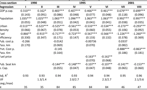
Table 3. OLS Regression results. Private transport energy consumption dependent variable.

Cross‐section 1990 1995 2001

Regression I II III IV V VI VII VIII

GDP p.cap. 0.310** (0.143) 0.162* (0.091) 0.483*** (0.086) 0.407*** (0.048) 0.466*** (0.077) 0.461*** (0.048) 0.679*** (0.118) 0.699*** (0.096) Population 1.035***

(0.055) 1.025*** (0.048) 1.065*** (0.051) 1.096*** (0.042) 1.063*** (0.041) 1.063*** (0.041) 0.992*** (0.038) 0.997*** (0.035) Urban density

‐0.513*** (0.066)

‐0.523*** (0.067) ‐0.525*** (0.078) ‐0.561*** (0.053) ‐0.533*** (0.060)

‐0.534*** (0.055)

‐0.273** (0.106)

‐0.293*** (0.092) Fuel

efficiency

‐0.866** (0.330)

‐0.915** (0.347) ‐0.717*** (0.171) ‐0.723*** (0.147) ‐0.567*** (0.133)

‐0.566*** (0.132)

‐1.226*** (0.378)

‐1.260*** (0.369) Pub. cost p.

Pass. km

‐0.266 (0.170)

‐0.0142 (0.069)

‐0.00736 (0.070)

0.0337 (0.082) Prvt. Cost p.

Pass. Km

‐0.145 (0.164)

‐0.888*** (0.186)

‐0.863*** (0.181)

Fuel price ‐0.163**

(0.070)

‐0.162** (0.068)

Pub. Seat km p. Cap.

‐0.144*** (0.055)

‐0.148*** (0.047)

‐0.107** (0.047)

‐0.107** (0.048)

‐0.141** (0.065)

‐0.153** (0.060)

Adj. R2 0.93 0.93 0.94 0.93 0.94 0.94 0.95 0.96 VIF

(avg./max)

1.3/1.4 2.0/2.7 2.3/2.7 2.1/3.6

N 35 35 84 85 84 84 46 47

Notes: White heteroscedasticity‐consistent standard errors in parentheses. Statistical significance is

(23)

[image:23.612.66.548.102.660.2]

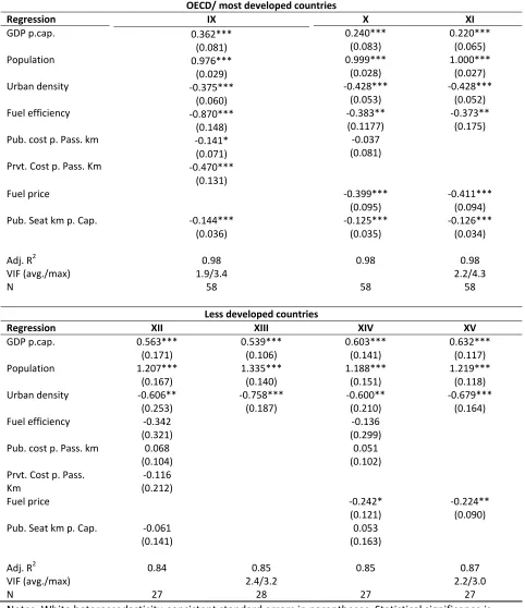
Table 4. OLS Regression results with the 1995 cross-section split according to

income/development level. Private transport energy consumption dependent variable.

OECD/ most developed countries

Regression IX

0.362*** (0.081) 0.976***

(0.029)

‐0.375*** (0.060)

‐0.870*** (0.148)

‐0.141* (0.071)

‐0.470*** (0.131)

X XI

GDP p.cap. 0.240***

(0.083)

0.220*** (0.065)

Population 0.999***

(0.028)

1.000*** (0.027)

Urban density ‐0.428***

(0.053)

‐0.428*** (0.052)

Fuel efficiency ‐0.383**

(0.1177)

‐0.373** (0.175) Pub. cost p. Pass. km ‐0.037

(0.081) Prvt. Cost p. Pass. Km

Fuel price ‐0.399***

(0.095)

‐0.411*** (0.094) Pub. Seat km p. Cap. ‐0.144***

(0.036) 0.98 1.9/3.4 58 ‐0.125*** (0.035) ‐0.126*** (0.034)

Adj. R2 0.98 0.98

VIF (avg./max) 2.2/4.3

N 58 58

Less developed countries

Regression XII XIII XIV XV

GDP p.cap. 0.563*** (0.171) 0.539*** (0.106) 0.603*** (0.141) 0.632*** (0.117) Population 1.207***

(0.167) 1.335*** (0.140) 1.188*** (0.151) 1.219*** (0.118) Urban density ‐0.606**

(0.253) ‐0.758*** (0.187) ‐0.600** (0.210) ‐0.679*** (0.164) Fuel efficiency ‐0.342

(0.321)

‐0.136 (0.299) Pub. cost p. Pass. km 0.068

(0.104)

0.051 (0.102) Prvt. Cost p. Pass.

Km

‐0.116 (0.212) Fuel price

‐0.242* (0.121)

‐0.224** (0.090) Pub. Seat km p. Cap. ‐0.061

(0.141)

0.053 (0.163)

Adj. R2 0.84 0.85 0.85 0.87

VIF (avg./max) 2.4/3.2 2.2/3.0

N 27 28 27 27

Notes: White heteroscedasticity‐consistent standard errors in parentheses. Statistical significance is

(24)

0.5 1 1.5 2 2.5 3 3.5 4 4.5 5

0 5,000 10,000 15,000 20,000 25,000 30,000 35,000 40,000 45,000

Ratio

city

per

capita

GDP

to

country

per

capita

GDP

[image:24.612.74.527.67.368.2]

Country per capita GDP (2001 USD/person)

Figure 1. The economic importance of cities. The ratio of city per capita GDP to the

(25)

R² = 0.63 0

20000 40000 60000 80000 100000

0 50 100 150 200 250 300 350

Private

transport

energy

use

per

capita

(MJ/person)

Urban density (persons/ha)

R² = 0.36

0 20000 40000 60000 80000 100000

20 30 40 50 60 70 80 90 100

Private

transport

energy

use

per

capita

(MJ/person)

[image:25.612.74.436.68.561.2]

National urbanization level

(26)

174 52

17

84

0 50 100 150 200 250

Asia (27) Europe (86) Aus, Can, US (38) ROW (16)

[image:26.612.75.543.70.353.2]

Average Urban Density (persons/ha)

(27)

Appendix Table A-1. Cities included in each dataset/cross-section.

1990 (35 total) 1995 (85 total) 2001 (47 total)

Boston Amsterdam Atlanta Amsterdam Brisbane Amsterdam Stockholm Chicago Brussels Calgary Athens Melbourne Athens Stuttgart

Denver Copenhagen Chicago Barcelona Perth Barcelona Turin Detroit Frankfurt Denver Berlin Sydney Berlin Valencia Houston Hamburg Houston Berne Wellington Bern Vienna Los Angeles London Los Angeles Bologna Bilbao Warsaw

New York Munich Montreal Brussels Bogota Bologna Zurich Phoenix Paris New York Budapest Cairo Brussels

San Francisco Stockholm Ottawa Copenhagen Cape Town Budapest Chicago Toronto Vienna Phoenix Dusseldorf Curitiba Copenhagen Dubai Washington Zurich San Diego Frankfurt Dakar Geneva Honk Kong

San Francisco Geneva Harare Ghent Melbourne Bangkok Adelaide Toronto Glasgow Johannesburg Glasgow Sao Paulo Hong Kong Brisbane Vancouver Graz Mexico City Graz Singapore

Jakarta Melbourne Washington Hamburg Rio de Janeiro Hamburg Kuala Lumpur Perth Helsinki Riyadh Helsinki

Manila Sydney Bangkok Krakow Sao Paulo Krakow Seoul Beijing London Tehran Lille Singapore Chennai Lyon Tel Aviv Lisbon

Tokyo Guangzhou Madrid Tunis London

Ho Chi Minh City Manchester Lyons

Hong Kong Marseille Madrid

Jakarta Milan Manchester

Kuala Lumpur Munich Marseilles

Manila Nantes Moscow

Mumbai Newcastle Munich

Osaka Oslo Nantes

Sapporo Paris Newcastle

Seoul Prague Oslo