Munich Personal RePEc Archive
Self-Attribution Bias and Consumption
Zinn, Jesse
30 September 2013
Online at
https://mpra.ub.uni-muenchen.de/50314/
Self-Attribution Bias and Consumption
Jesse Aaron Zinn
∗University of California Santa Barbara
September 30, 2013
Abstract
In this paper I examine the implications of self-attribution bias on
con-sumption and savings decisions. When self-attributive learning replaces
rational expectations in a model of intertemporal choice, two departures
from the permanent-income hypotheses manifest. One is that consumers
tend to under-save early in life. Another is a relatively high degree of
co-variance between changes in consumption and changes in income. No other
factor on its own has been able to explain both of these empirical anomalies
that the permanent-income hypothesis has faced.
JEL Codes: D03, E21
Keywords: Cognative Biases, Uncertainty, Consumption, Saving
1
Introduction
Self-attribution bias refers to the tendency to credit one’s self for desirable
out-comes while blaming undesirable outout-comes on external factors.1 For example, a ∗
I am grateful to Javier Birchenall, Gary Charness, Zack Grossman, and seminar discussants at the 2013 conference of the Society for the Avdancement of Behavior Economics for their comments and suggestions.
1See Taylor and Brown (1988) or Campbell and Sedikides (1999) for surveys on the subject
professional athlete who exhibits the bias may blame his coaches, teammates, the
referees, or “bad luck” for poor performance, rather than his own lack of ability.
There has been some work in economics and finance that considers self-attribution.
Daniel, Hirshleifer, and Subrahmanyam (1998) theorize that self-attribution bias
and over-confidence account for excess volatility in securities markets relative to
that implied by models with fully rational decision makers. Gervais and Odean
(2001) present a model wherein traders are initially ignorant of their ability but
tend to become overconfident over time due to self-attribution. Choi and Lou
(2010) find that self-attribution bias affects the decisions of mutual fund
man-agers, and that it leads to poor performance. Interestingly, they find biased
self-attribution amongst younger managers but little evidence for it among more
experienced mutual fund managers.
The present study considers the effects of self-attributive learning on decisions
involving consumption spending and savings. Self-attribution may be relevant
to consumption/savings decisions because it is thought to be a mechanism by
which individuals bolster their self-esteem (Shepperd, Malone, and Sweeny, 2008).
If consumers buoy their self-esteem by believing they will earn relatively high
incomes over their lifetime (as a result of self-attribution bias) then this should
affect their consumption/savings decisions as well, since such decisions are thought
to be based upon expectations regarding future income.
This study details two implications of self-attribution bias on the dynamics of
consumption spending. One implication is that consumption tends to be
unsus-tainably high early in life, leading to a probable decrease in consumption later
in life. Hence, self-attribution bias can be used to explain the fact that many
individuals and households over-consume and under-save. Another implication of
with changes in income under self-attribution bias than for rational expectations.
So, self-attributive learning explains the “excessive sensitivity” (Flavin, 1981) of
consumption to income found in empirical analyses.
The intuition behind over-consumption early in life is that self-attribution bias
tends to entail optimistic expectations for future earnings and an
overly-optimistic individual will consume more early in life because he or she expects
to finance such spending with greater earnings in future periods. Relative to
a consumer with rational expectations, the greater degree of covariation between
changes in consumption and changes in income for a consumer with self-attribution
bias stems from the fact that income in any period provides a signal about the
likelihoods of future incomes for the self-attributor but not for the consumer with
rational expectations, the latter of whom inherently knows the probabilities of
any level of income in any future period.
It is well-known that there is no single factor that has been able to explain both
of these phenomena.2 For example, hyperbolic discounting on its own generates
over-consumption, but it requires at least one other non-standard assumption
(such as credit constraints) in order to account for greater covariation between
changes in consumption and changes in income (Angeletos, Laibson, Repetto,
Tobacman, and Weinberg, 2001). Thus, self-attribution bias represents a more
parsimonious theory of consumption that diverges from the permanent-income
hypothesis in these ways.
There is some empirical evidence that may corroborate with the theory
pre-sented in this paper. Kooreman, Prast, and Vellekoop (2009) find significantly
different propensities to save for wages that were labelled differently on the
pay-checks of employees at a Bank and an insurance company in The Netherlands. In
2
particular, people saved a lower proportion of a “performance bonus” than they
did a “vacation allowance” or a “13th month”. They explain this finding using
the mental accounting framework, that there could be “a mental accounting
re-lationship between the label of an income component and how the component is
put to use”.3 Self-attribution bias could be another explanation for the findings
regarding performance bonuses. If employees treat performance bonuses as a
sig-nal of their own high ability then they will expect to earn more bonuses in the
future, and they will consume more and save less of this extra income than they
would have otherwise.
The remainder of the paper is organized as follows: Section 2 discusses other
theories of consumption, and how the present work aims to fill a gap in the
literature. Section 3 presents and analyzes an intertemporal consumption and
savings model with self-attributive learning. Section 4 concludes.
2
Theories of Consumption
This section offers a discussion of the various theories of consumption. The
pur-pose of the section is to identify the gap in our understanding of consumption and
savings decisions that this work fills.
The theory of aggregate consumption has a history dating back at least to
Keynes (1936), who conjectured that consumption in any period depends
primar-ily on income for that period and that other variables have only negligible effects
on consumption. A controversial property of Keynes’s consumption function is
that the average propensity to consume (i.e. the ratio of consumption to income)
decreases as income grows. Although empirical analyses of cross-sections
sup-3Thaler (1980) initiated the mental accounting literature. See Thaler (2004) for fairly recent
ported the idea of decreasing average propensity to consume, time-series analyses
suggested that the ratio is fairly constant despite substantially growing incomes
over long periods of times.4 These empirical failures of the Keynesian
consump-tion funcconsump-tion begat a search for new theories of consumpconsump-tion. The most influential
substitutes were a pair of related, neoclassical hypotheses: the life-cycle
hypoth-esis of Modigliani and Brumberg (1954) and the permanent-income hypothhypoth-esis of
Friedman (1957). These theories emphasized real wealth, including discounted
future real income, as the determinant of consumption. When coupled with the
rational expectations hypothesis these theories imply that consumption
fluctu-ates relatively little compared to contemporaneous income, that consumption is
smooth.5
However empirical evidence suggests that consumption is not as smooth as
these hypotheses imply. For example, Campbell and Mankiw (1990) find that
about half of consumption spending is determined by contemporaneous income
while the rest is determined by other variables. Wilcox (1989), Shea (1995),
Banks, Blundell, and Tanner (1998), Parker (1999), Souleles (1999), and
Bern-heim, Skinner, and Weinberg (2001) find evidence that consumption depends more
on contemporaneous income than implied by the permanent-income hypothesis.
In a similar vein of research, Carroll (1994) provides evidence that consumption
is a poor indicator of future income and Startz (2008) finds that lagged income is
a much better predictor of future income than present consumption.
There have been a number of theories proposed to explain the apparent lack
of smoothness in consumption implied by rational expectations and the life-cycle
4Perhaps the most noteworthy example of this empirical work is Kuznets (1946).
5Hall (1978) shows that the permanent-income hypothesis coupled with rational expectations
and permanent-income hypotheses. Neoclassical theory typically assumes that
consumers have preferences only over their consumption. Some studies have
re-laxed this assumption, and considered preferences over sociological phenomena.
The concepts ofconspicuous consumption and pecuniary emulation from Veblen
(1899) involve preferences to signal wealth through consumption. In the
expo-sition of the relative-income hypothesis, Duesenberry (1949) reasons that these
phenomena lead to lower levels of saving than would occur if consumers only had
preferences over consumption. Another sociological theory is proposed by Akerlof
(2007), who argues that there is a socialnorm whereby individuals feel entitled to
spend their current income (and under-save), a norm that could be modelled by
a direct preference to save less. A behavioral approach involves time-inconsistent
preferences in the form ofhyperbolic discounting, wherein, at a given point in time,
consumption in the present is more valued than the next period by a greater factor
than consumption in future proximate periods.6
The present study adds to this list of theories that attempt to explain
con-sumption patterns. A notable difference between the theory presented herein and
previous alternatives to the fully rational model is that it focuses on irrationality
with respect to the beliefs agents hold, whereas previous theories dealt with
pref-erences that were in, in one sense or another, non-standard. An implication of
this is that previous theories typically utilize the rational expectations hypothesis,
whereas the present study does not (except as a basis for comparison).
To summarize, the theories of consumption that have been offered as an
al-ternative to the permanent income hypothesis have heretofore dealt with
non-standard preferences drawn from the fields of psychology and sociology. This
6
work differs from these theories in that it focuses on non-standard beliefs, which
tend to be biased in a systematic manner. A complete theory of consumption
would utilize realistic preferencesand beliefs, so this work complements previous
theories by moving our understanding closer to that goal.
From a policy perspective, it is important to consider the multitude of
expla-nations for a given phenomenon so that efforts to improve economic outcomes
are not doomed to failure simply because our understanding is incomplete. For
example, if self-attribution bias is a major reason for why some people under-save,
then a policy designed to induce time-consistent discounting of future
consump-tion may not be cost effective for attaining the underlying goal of getting people
to not under-save. Therefore, this work has value to policy-makers by giving them
a more complete understanding of consumption spending, and how it might be
influenced.
3
Self-Attribution and Intertemporal Choice
This section presents a model designed to obtain implications of embedding
self-attributive learning in an otherwise conventional consumption and savings model.
Consider an economy in which individuals earn income in each of T periods,
1, . . . , T and decide how much to consume in each ofT +R periods 1, . . . , T+R,
whereRis the number of periods spent in retirement. Denote the random variable
representing consumer i’s income in period t with yit.
Let cit denote consumer i’s consumption spending in period t. Assume that
each consumer’s preferences over (ci1, . . . , ciT+R) satisfy the expected utility
maximizing
E
"T+R X
t=1 cit−
γc2 it
2
#
, (1)
with γ > 0 and sufficiently small to guarantee that marginal utility is positive
over relevant values of cit.
A quadratic period utility function, zero discount rate, and zero interest rate
are used in order to focus exclusively on how consumption changes due to changes
in beliefs. Generally, consumers choose levels of consumption in order to equalize
the present value of discounted marginal utility. Quadratic utility is unique in
that it implies that consumption is equal to the expected value of consumption
in future dates,7 which is equal to the average level of income the individual
expects to earn over the remaining periods in life. As such, these results generalize,
somewhat, to any monotonically increasing utility function since they all imply
that consumption is increasing in expected average income. Besides, if this were
not the case then consumption would change over time even if beliefs did not
change, simply because of one’s attitude toward risk and the decrease in the
riskiness of total lifetime income as time passes. Similarly, if the discount factor
and interest rate were non-zero they would generally interact to affect consumption
levels. If these factors were present in the analysis then determining the extent
to which fluctuations in consumption were due to changes in expectations would
be muddled by attitudes toward risk and the interplay between the discount and
the rate of interest, so the confounding factors are eliminated.
7
To see this, note that a first-order condition for a general utility function u is u′
(cit) =
Et[u′(cit+1)]. Whenuis quadraticu′ is linear, so the condition becomes u′(cit) =u′(Et[cit+1])
Consumer i’s lifetime budget constraint is
T+R
X
t=1 cit =
T
X
t=1
yit, (2)
where equality is ensured by the assumption that the marginal utility of each
period’s consumption is positive.
Let Et denote the general expectation operator given information up to time
t.8 For consumer i choosing how much to consume in period t the optimality
conditions for maximization of expression (1) are
cit =Et[ciτ], for all τ ∈ {t+ 1, . . . , T}. (3)
Each consumer will expect, at each period t, that lifetime income will eventually
be spent, so
t−1
X
τ=1 ciτ +
T+R
X
τ=t
Et[ciτ] = t−1
X
τ=1 yiτ +
T
X
τ=t
Et[yiτ]. (4)
Here it is important to emphasize that in this model there is no credit constraint
on any individual, so it is possible for cit> yit in any period t.
From expression (3), Substitutecit for each Et[ciτ] term in expression (4) and
solve for cit to obtain
cit=
1
T +R−t+ 1
t−1
X
τ=1
yiτ −ciτ + T
X
τ=t
Et[yiτ]
!
, (5)
which says that consumption in any period t is equal to accumulated savings
(Pt−1
τ=1yiτ −ciτ) plus expected income from the current period on (P T
τ=tEt[yiτ]),
divided by the number of remaining periods in which consumption will take place
8
Information for consumeriup to timetis essentially having observed the realized values of
(T +R−t+ 1).
3.1
Self-Attribution and Expectations
Suppose income in each of the non-retirement periods take one of two possible
values: y′
and y, with y′
> y. Let θi ∈(0,1) denote the probability that yit =y′
for any i and all t. As θi is the probability of earning the higher level of income,
we can interpretθi as a measure of i’s income earning ability.
We will focus on the case in which consumers do not know their values ofθi (so
explicitly assuming that consumers do not hold rational expectations, under which
θi is known by each i). Consumers will instead infer the value of θi by observing
their income levels. These inferences will be modelled with the weighted updating
model studied in Zinn (2013), which is a generalization of Bayes’ rule that allows
for biased belief formation. Therefore, beliefs regardingθigiven the realized values
yi1, . . . , yit, for each period t, are summarized by
˜
πit(θi|yi1, . . . , yit) =
π(θi)Qtτ=1f(yiτ|θi)ψ(yiτ)
R1
0 π(θi)
Qt
τ=1f(yiτ|θi)ψ(yiτ)dθi
, (6)
where each f(yiτ|θi) is the likelihood function associated with income yiτ and π(θi) is the prior distribution. The weighting function ψ : {y, y
′
} → R+ gives
a measure of how informative individual i regards the observed level of income.
9 As Bayesian updating is the case when all weights equal one, the consumer
is respectively treating an observation of income yiτ as less, equally, or more
informative compared to a perfect Bayesian if the weightψ(yiτ) is less than, equal
9Results from Zinn (2013) show that larger values ofψlead to the effective likelihood function
proportional to f(zi|θi)ψ having less information entropy as ψincreases. That ψ is a measure
to, or greater than one.
Self-attribution bias involves associating undesirable outcomes with luck while
ascribing desirable outcomes to internal, personal factors (such as ability), so
as-sume that conas-sumers blame luck when yit = y and that they attribute yit = y
′
to their ability. To dismiss an outcome as being due to luck is to consider that
outcome as not being very informative, which is modelled with a low weight
rel-ative to that of a Bayesian. So, ψ(y) = δ ∈ [0,1). The theory of self-attribution bias posits that those who exhibit the bias ascribe positive outcomes to ability.
How this translates to restrictions we ought to place on ψ(y′
) is unclear, except
that it must be the case that ψ(y′
) > ψ(y). So simply assume that ψ(y′
) = 1,
the minimum value of the range suggested by theory. In essence, this assumption
stipulates that self-attribution bias involves putting as much weight on the
desir-able outcome as a perfect Bayesian updater would, implying that the irrational
learning is driven entirely by the under-weighting of undesirable outcomes.
Eachyit is a Bernoulli trial with parameterθi, so the likelihood functions may
be expressed as
f(yit|θi) =
θi if yit =y′
(1−θi) if yit =y.
Assume that each consumer i’s prior distributionπ(θi) is from the beta family of
distributions, with parameters ai, bi ∈R++. That is
π(θi) =
θai−1
i (1−θi)bi−1
R1
0 θ ai−1
i (1−θi)bi−1dθi
This ensures tractability as beta distributions are the conjugate priors of the
bi-nomial distribution, ensuring that posterior distributions are in the beta-bibi-nomial
Let zit denote the number of times consumer i has observed the high income
levely′
in the firstt periods. Then the weighted updating model expressed in (6)
can be restated more specifically:
˜
π(θi|yi1, . . . , yit) =
θzit+ai−1
i (1−θi)δ(t−zit)+bi−1
R1
0 θ
zit+ai−1
i (1−θi)δ(t−zit)+bi−1dθi .
Assume consumers use the (subjective) expected value ofθias point estimates.
Then after observing income levels in the first t periods, consumer iwill estimate
θi to be
˜
θit ≡E˜(θi|yi1, . . . , yit)
≡
Z 1
0
θiπ˜(θi|yi1, . . . , yit)dθi
= ai+zit
ai+bi+δt+ (1−δ)zit
. (7)
(A full derivation of the formula for ˜θit in expression (7) is presented in the
ap-pendix.)
A notable aspect of ˜θit is how it tends to behave as the number of observations
increases without bound. Notice that
lim
t→∞
˜
θit = lim
t→∞
ai+zit
ai +bi+δt+ (1−δ)zit
= lim
t→∞
ai+tθi
ai +bi+δt+ (1−δ)tθi
= lim
t→∞
ai
t +θi ai+bi
t +δ+ (1−δ)θi
= θi
δ+θi−δθi
(8)
where the inequality in the final line is a consequence of δ, θi ∈ (0,1) implying
thatδ+θi−δθi−1 = (1−θ)(δ−1)<0, from which it follows thatδ+θi−δθi <1.
That limt→∞θ˜it> θi suggests that with self-attribution bias any consumer, given
enough observations, will (i.e. with sure convergence) eventually become more
optimistic than counterparts with rational expectations. Thus, one would expect
that ˜θit will grow over time.
It is not true that ˜θit+1 > θ˜it for every consumer i and in every period t.
That depends on the actual observations; if a consumer repeatedly observes the
low income level y then he or she will not grow more optimistic. Whether or
not ˜θit increases also depends on the prior distribution. For example, if the prior
distribution is overly optimistic (particularly when ai
ai+bi > limt→∞ ˜
θit) then ˜θit
will tend to decrease as it converges to θi
δ+θi−δθi.
The estimator ˜θit will generally be biased by the prior distributionπ(θi), even
in the case where δ = 1, and the consumer updates according to Bayes’ rule.
In order to study only the bias due to self-attributive learning, this analysis will
focus exclusively on cases where the prior distribution does not generate bias by
imposing that ai
bi =
θi
1−θi, so the prior distribution is accurate in the sense that E(˜θi0) = θi. Then any remaining bias in the estimate ˜θit will be due to
self-attribution. To achieve this, do the following: for anyk > 0, substitutekθi forai
andk(1−θi) forbi, so that abii = 1−θiθi. Now, impose that consumeriexperiences an approximately typical history, by substituting tθi =E(zit|θi) for zit in expression
(7). Define the beliefs from such an approximately typical experience as
¯
θit ≡
kθi+tθi
kθi+k(1−θi) +tθi+δ(t−tθi)
= θi(k+t)
k+δt+tθi(1−δ)
To understand how these beliefs tend to change over time, take the time derivative
of expression (9):
∂θ¯it ∂t =
kθi(1−θi)(1−δ)
[k+δt+tθi(1−δ)]2
>0. (10)
That this derivative is positive shows that self-attribution bias will tend to induce
increasingly optimistic beliefs (up to a limiting value) as time passes.10 To
reiter-ate, this result suggests that when the bias introduced by the prior distribution
is eliminated, beliefs regarding the value of θi will typically rise over time.
3.2
Self-Attribution and Consumption
The previous subsection established that beliefs generated with self-attribution
tend to become increasingly optimistic over time, increasing surely (in the
tech-nical sense) as the number of observations increases without bound. The present
subsection analyzes how these beliefs affect consumption over time.
Substituting ˜θity
′
+ (1−θ˜it)yfor Et[yiτ] for allτ ≥t in expression (5) yields11
cit =
1
T +R−t+ 1
t
X
τ=1 yiτ −
t−1
X
τ=1 ciτ +
T
X
τ=t
˜
θity
′
+ (1−θ˜it)y
!
=
Pt
τ=1yiτ −P
t−1
τ=1ciτ + (T −t+ 1)[˜θity′+ (1−θ˜it)y] T +R−t+ 1
To illustrate this pattern of consumption the analysis will utilize a numerical
example, in which the parameter values are as follows: T = 40 periods of time
over which income is earned and there are R = 10 periods of retirement where
consumption takes place and income is not earned. Low income y = 10, high
income y′
= 15, and each are equally likely in each period, so θi = 1/2. Prior
10Note that the time derivative is zero under Bayesian updating (when δ = 1), suggesting
that beliefs will tend to stay constant over time for such a consumer.
11Note also the substitutiony
distribution parameters areai =bi = 1, so the prior is a uniform distribution over
[0,1]. Importantly, in light of the discussion at the end of the last subsection,
the expected value of θi given this uniform prior is 1/2, so the prior estimate is
accurate and bias due to the prior distribution’s affect on subsequent estimates is
eliminated. The combination ofθi =1/2and ai =bi = 1 implies that k =1/2. The
weight consumers put on the likelihood functions associated with the low income
level isδ=1/2, which, since it is less than one, is what drives self-attribution and
optimism bias that occurs in this example.
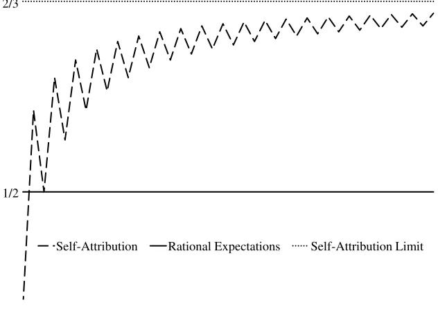
Because it offers clearer insight than a random sequence, consider the case
where the income levels y = 10 and y′
= 15 alternate from period to period,
starting with yi1 = y. As the initial income level is low and the weight on that
observation is positive, the first-period estimate ˜θi1 =2/5<1/2=θi and one could
say that the consumer with self-attribution bias is actuallypessimistic in the first
period.12 This pessimism quickly subsides as the estimate rises substantially in the
next period to ˜θi2 =4/7, falls to ˜θi3 =1/2, then rises again, remaining greater than
the true valueθi =1/2, and tending toward the limiting value limt→∞θ˜it =2/3.13 As
such, after the initial period the consumer with self-attribution bias who witnesses
this sequence will never believe that the high level of income is less likely than
the low level of income, despite the fact that the number of periods during which
income is high never outnumbers the number of periods in which income was low.
Figure 1 shows this sequence of beliefs graphically, with time going increasing
from left to right, alongside the analogous beliefs of a consumer with rational
expectations (i.e. one who knows thatθi =1/2). The local maxima (corresponding
12Though, compared to a perfect Bayesian with identical priors (who estimates θ
i to be1/3),
this consumer with self-attribution is not as pessimistic as he or she “should” be.
13From expression (8), lim
t→∞θ˜it = δ+θθii−δθi. Substituting the numerical values yields
0.5
Figure 1: Estimates of θi over the First Forty Periods of Life
Self-Attribution Rational Expectations Self-Attribution Limit 1/2
2/3
to when the time index is even-numbered) on the graph for beliefs formed under
self-attribution coincide with the approximately typical set of beliefs ¯θit because
at those points it is true that zit = θit. Notice that these local maxima increase
monotonically, in agreement with the findings of expression (10).
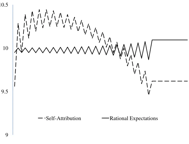
Figure 2 depicts the sequence of consumption levels corresponding to this
alternating sequence of income levels for both a consumer with self-attribution
bias and a consumer with rational expectations. As the consumers in this example
both earn each of the income levels in 20 periods each during the 40 years of
pre-retirement, lifetime income and consumption for these consumers is 500 units.
This consumption is spread over 50 periods during which consumption can take
place, so consumption will average 10 units per period. As these consumers both
Figure 2: Lifetime Consumption Profiles
9 9.5 10 10.5
Self-Attribution Rational Expectations
around this level of 10 units of consumption.
A glaring disparity between the consumption sequences depicted in Figure 2 is
that the consumer with rational expectation has consumption levels that fluctuate
consistently about the average level of 10 while the self-attributor has consumption
that fluctuates above 10 for low t (other than the first period, because income in
that period is low) but then fluctuates below 10 for high t. There is another
disparity that is related to the one just mentioned: the rational consumer enjoys
a higher level of consumption in retirement than the self-attributor.
These disparities occur because self-attribution bias tends to lead to
overly-optimistic expected income in the future, inducing consumers to consume at levels
that are not likely to be sustainable. These levels of consumption require the
smooth income throughout life, possibly driving the consumer to incur debt which
must be paid back. Such low savings early in life will likely necessitate that
spend-ing levels fall later on. Takspend-ing another look at expression (5), for the consumer
with self-attribution bias the expression for savingsPt−1
τ=1yiτ−ciτ will tend to be
lower than for the rational consumer, likely causing a drag on consumption and
causing it to decrease when after enough time passes and the reality of
less-than-anticipated lifetime income sets in. As such, self-attribution bias offers a novel
explanation for under-saving and low levels of consumption in retirement.
3.3
Period-to-Period Variation in Consumption
As depicted in Figure 2, these consumption sequences both vary with income
levels from period to period. For the consumer with rational expectations, this
covariation occurs through one channel, the “direct wealth effect.” The direct
wealth effect is the change in consumption due to actual income in any given
period differing from its expected level. Holding expectations constant, expected
lifetime earnings changes by this exact amount. Therefore, for an individual with
rational expectations who intends to perfectly smooth consumption over a lifetime,
consumption from one period to the next will change by the difference between
actual income and expected income in that period divided by the number of
periods left in which to consume. This is readily apparent by subtracting the
periodt version of expression (5) from the period t+ 1 version14
cit+1−cit =
1
T +R−t T
X
τ=t+1
Et+1[yiτ]−Et[yiτ]
!
, (11)
then substituting the newly-observed valueyit+1 forEt+1[yit+1], and imposing that
expectations for the observations of future income levels do not change (as is the
case with rational expectations), so that Et+1[yiτ] = Et[yiτ] for τ > t + 1, to
conclude
Rational Expectations =⇒ cit+1−cit =
yit+1−Et[yit+1]
T +R−t . (12)
For the consumer with rational expectations depicted in Figure 2, taking the
absolute value of expression (12) while substituting the numerical values for the
relevant terms yields |cit+1 −cit|= 502.−5t, from which it is clear that consumption
fluctuates with greater magnitude as time passes (as t increases, going from left
to right in Figure 2). The interpretation of this is that the difference between
the actual income and expected income each period is divided into less remaining
periods as time passes.
In contrast, the consumer who forms belief through self-attribution has
con-sumption levels that vary with income through an additional channel: the
“up-dated beliefs effect”. This accounts for the effect of the newly-observed level of
income on beliefs. For example, if this consumer earns high income (in any period
t < T = 40) then lifetime expected wealth will increase by that amount, minus
the expected level of income for that period, plus the increase in expected future
income due to the change in beliefs due to this observation. To see this
mathemat-ically, take expression (11) and, to emphasize that these are expectations formed
through self-attribution bias, substitute
˜
Et[yiτ]≡θ˜ity
′
forEt[yiτ] and then substitute yit+1 for ˜Et+1[yit+1]. These yield
cit+1−cit =
yit+1−E˜t[yit+1]
T +R−t +
PT
τ=t+2E˜t+1[yiτ]−E˜t[yiτ]
T +R−t . (13)
The term
yit+1−E˜t[yit+1]
T +R−t (14)
in expression (13) is the direct wealth effect and the term
PT
τ=t+2E˜t+1[yiτ]−E˜t[yiτ]
T +R−t (15)
represents the updated beliefs effect.
Because income affects consumption through an additional channel (the
up-dated beliefs effect) for the consumer with self-attribution bias, one might expect
that changes in consumption and changes in income have a higher degree of
co-variance for this consumer relative to the rational consumer. Indeed this is the
case, as the covariance between changes in income and changes in consumption
for the self-attributor is 0.812 and for the rational consumer it is 0.396.
Consider the direct wealth effect for the consumer with self-attribution bias in
expression (14). From expression (10), ˜Et[yit+1] tends to increase as the consumer
with self-attribution bias becomes increasingly optimistic with additional
observa-tions. This tends to make the direct wealth effect weaker when the income level is
high than the decrease in consumption when income is low. And this phenomenon
gets stronger as time proceeds, both because of the fact that ˜Et[yit+1] tends to
increase and the fact that there are fewer time periods over which to spread the
discrepancies between observed income and expected levels of income. One can
large, as consumption tends to decrease overall.
The updated beliefs effect works somewhat differently than the direct wealth
effect. For additional clarity, utilize the fact that this effect can be rewritten
PT
τ=t+2E˜t+1[yiτ]−E˜t[yiτ]
T +R−t =
T +R−t−1
T +R−t (˜θit+1−θ˜it)(y
′
−y)
As t increases: T+R−t−1
T+R−t decreases and, since ˜θit is bounded and converges to 2/3
for the parameter values used in this example, ˜θit+1−θ˜it tends to decrease as the
consumer becomes more optimistic at a slower rate.15 Thus, the updated beliefs
effect is greater for relatively low t. Also, because of the nature of self-attribution
bias, ˜θit+1−θ˜itwill increase more in a period when income is high than it decreases
when income is low. This fact is what drives θit to tend to grow over time, and
one can see it clearly in Figure 1 where any downward movement in θit is always
smaller than the immediately subsequent upward movement. Together, these facts
imply that the updated beliefs effect results in larger magnitudes for the changes
in consumption for low t, with increases being larger than decreases.
In combination, the direct wealth effect and the updated beliefs effect imply
that consumption for the individual with self-attribution bias will tend to rise early
in life (for low t) and decline later in life (for high t). Thus, these phenomena,
which themselves are implied by self-attributive learning, tend to cause
over-consumption.16
15One can also argue that ˜θ
it+1−θ˜ittends to decrease because ¯θitis monotonically increasing
and strictly concave.
16It is interesting to note that parsing of the change of consumption into the direct wealth
effect and the updated beliefs effect obscures the phenomenon of under-saving until one considers how the direct wealth effect and the updated beliefs effect play out over the lifetime. The under-saving explanation for the broader consumption pattern was obscured in the analysis of period-to-period changes in consumption by the fact that the changes in savings from one period to the next are relatively small, and one can see this mathematically as the savings terms
Pt−1
τ=1yiτ−ciτ andPtτ=1yiτ−ciτ largely cancel each other out (i.e. they “telescope” away) in
4
Concluding Remarks
In this study, I show that self-attribution bias leads to two well-known phenomena
that are inconsistent with the permanent-income hypothesis: under-saving and
excess sensitivity of consumption to income. Because previous explanations of
these two phenomena require multiple factors, it is noteworthy that they can now
be explained by a single factor embedded within a standard intertemporal choice
model. Thus, not only does self-attributive learning represent a novel theory that
is capable of explaining some of the most notable stylized facts about consumption,
but it also embodies a theory that is more parsimonious than alternatives.
I believe that these theoretical findings warrant empirical investigation. A clear
method of testing the theory would be to look at data on performance bonuses
and measuring the propensity to consume such bonuses versus income with other
labels, as is done in Kooreman, Prast, and Vellekoop (2009). So that there is
plenty of opportunity for employees to mistakenly credit themselves for desirable
outcomes, it would be particularly valuable to investigate industries in which it
is difficult to determine whether performance is due to an employee’s ability or
outside factors. An example is the performance bonuses of professional traders,
who may seem to do well because the broader stock market increases, or simply
Appendix
Deriving the Expression for
θ
˜
itIn the following derivation, Γ denotes the gamma function, B denotes the beta
function, and we make use of the properties
Γ(r+ 1) =rΓ(r) and B(r, s)≡ Γ(r)Γ(s)
Γ(r+s)
for all r, s∈R++. Now,
˜
θit ≡E˜(θi|yi1, . . . , yit)
≡
Z 1
0
θiπ˜(θi|yi1, . . . , yit)dθi
=
Z 1
0
θzit+ai
i (1−θi)δ(t−zit)+bi−1
R1
0 θ
zit+ai−1
i (1−θi)δ(t−zit)+bi−1dθi dθi
= B(zit+a+ 1, δ(t−zit) +b)
B(zit+a, δ(t−zit) +b)
= Γ(zit+a+ 1)Γ(δ(t−zit) +b) Γ(zit+a+ 1 +δ(t−zit) +b)
∗ Γ(zit+a+δ(t−zit) +b)
Γ(zit+a)Γ(δ(t−zit) +b)
= Γ(zit+a+ 1) Γ(zit+a)
∗ Γ(zit+a+δ(t−zit) +b))
Γ(zit+a+ 1 +δ(t−zit) +b)
= ai+zit
Deriving the Expression for
∂θ¯it∂t
∂θ¯it ∂t =
∂ θi(k+t)
k+δt+tθi(1−δ) ∂t
= θi[k+δt+tθi(1−δ)]−θi(k+t)[δ+θi(1−δ)] [k+δt+tθi(1−δ)]2
= θi[k+δt+tθi(1−δ)−(k+t)(δ+θi(1−δ))] [k+δt+tθi(1−δ)]2
= θi[k−kδ−kθi(1−δ)] [k+δt+tθi(1−δ)]2
= kθi[1−δ−θi(1−δ)] [k+δt+tθi(1−δ)]2
= kθi(1−θi)(1−δ) [k+δt+tθi(1−δ)]2
.
Deriving the Expression for
c
it+1−
c
itThe periodt+ 1 version of expression (5) is
cit+1 =
1
T −t t
X
τ=1
yiτ −ciτ + T
X
τ=t+1
Et+1[yiτ]
!
. (16)
To obtain an expression forcit+1−cit, one can add and subtract the sumPTτ=tEt[yiτ]
within expression (16) to obtain
cit+1 =
1
T −t t
X
τ=1
yiτ −ciτ + T
X
τ=t
Et[yiτ] + T
X
τ=t+1
Et+1[yiτ]− T
X
τ=t
Et[yiτ]
!
pull yit −cit from Ptτ=1yiτ −ciτ and yit from PTτ=tEt[yiτ], and then utilize
ex-pression (5) to substitute in (T −t+ 1)cit, yielding
cit+1 =
1
T −t (T −t+ 1)cit+yit−cit−yit+ T
X
τ=t+1
Et+1[yiτ]−Et[yiτ]
!
=cit+
1
T −t T
X
τ=t+1
Et+1[yiτ]−Et[yiτ]
!
,
which implies that
cit+1−cit=
1
T −t T
X
τ=t+1
Et+1[yiτ]−Et[yiτ]
!
.
References
Akerlof, G. A. (2002): “Behavioral Macroeconomics and Macroeconomic
Be-havior,” American Economic Review, 92(3), 411–433.
(2007): “The Missing Motivation in Macroeconomics,” American
Eco-nomic Review, 97(1), 3–36.
Angeletos, G.-M., D. Laibson, A. Repetto, J. Tobacman, and
S. Weinberg (2001): “The Hyperbolic Consumption Model: Calibration,
Simulation, and Empirical Evaluation,”The Journal of Economic Perspectives,
15(3), 47–68.
Banks, J., R. Blundell, and S. Tanner (1998): “Is There a
Retirement-Savings Puzzle?” American Economic Review, 88(4), 769–788.
Variation in Retirement Wealth among US Households?” American Economic
Review, 91(4), 832–857.
Campbell, J., and N. Mankiw (1990): “Permanent Income, Current Income,
and Consumption,” Journal of Business & Economic Statistics, 8(3), 265–279.
Campbell, W. K., and C. Sedikides (1999): “Threat Magnifies the
Self-Serving Bias: A Meta-Analytic Integration,” Review of General Psychology,
3(1), 23-43.
Carroll, C. D. (1994): “How Does Future Income Affect Current
Consump-tion?” The Quarterly Journal of Economics, 109(1), 111–147.
Choi, D., and D. Lou (2010): “A test of the Self-Serving Attribution Bias:
Evidence from Mutual Funds,” in Fourth Singapore International Conference
on Finance.
Daniel, K., D. Hirshleifer,and A. Subrahmanyam(1998): “Investor
Psy-chology and Security Market Under-and Overreactions,” Journal of Finance,
53(6), 1839–1885.
Duesenberry, J. S. (1949): Income, Saving, and the Theory of Consumer
Be-havior. Harvard University Press.
Flavin, M. A. (1981): “The Adjustment of Consumption to Changing
Expecta-tions about Future Income,” The Journal of Political Economy, pp. 974–1009.
Frederick, S., G. Loewenstein, and T. O’Donoghue (2002): “Time
Dis-counting and Time Preference: A Critical Review,” Journal of Economic
Friedman, M. (1957): A Theory of the Consumption Function. Princeton
Uni-versity Press.
Gervais, S., and T. Odean (2001): “Learning to Be Overconfident,” Review
of Financial Studies, 14(1), 1–27.
Hall, R. E. (1978): “Stochastic Implications of the Life Cycle-Permanent
In-come Hypothesis: Theory and Evidence,” Journal of Political Economy, 86(6),
971–987.
Keynes, J. M. (1936): The General Theory of Employment, Interest, and
Money. MacMillon, New York.
Kooreman, P., H. Prast, and N. Vellekoop (2009): “Labeling, Frequency
and Default Effects in an Employee Savings Scheme,” University of Tilburg
Working Paper.
Kuznets, S. (1946): National Product Since 1869. National Bureau of Economic
Research, New York.
Laibson, D. (1997): “Golden Eggs and Hyperbolic Discounting,” The Quarterly
Journal of Economics, 112(2), 443–478.
Modigliani, F., and R. Brumberg (1954): “Utility Analysis and the
Consumption Function: An Interpretation of Cross-Section Data,” in
Post-Keynesian Economics, pp. 388–436. Rutgers University Press.
Parker, J. A.(1999): “The Reaction of Household Consumption to Predictable
Changes in Social Security Taxes,”American Economic Review, 89(4), 959–973.
Shea, J. (1995): “Union Contracts and the Life-Cycle/Permanent-Income
Hy-pothesis,” American Economic Review, 85(1), 186–200.
Shepperd, J., W. Malone,and K. Sweeny(2008): “Exploring Causes of the
Self-serving Bias,” Social and Personality Psychology Compass, 2(2), 895–908.
Souleles, N. S. (1999): “The Response of Household Consumption to Income
Tax Refunds,” American Economic Review, 89(4), 947–958.
Startz, R. (2008): “Are Consumers Forward-Looking?,” University of
Wash-ington, Department of Economics Working Papers.
Taylor, S. E., and J. D. Brown (1988): “Illusion and Well-Being: A Social
Psychological Perspective on Mental Health,” Psychological Bulletin, 103(2),
193-210.
Thaler, R. H.(1980): “Toward a Positive Theory of Consumer Choice,”Journal
of Economic Behavior & Organization, 1(1), 39-60.
(2004): Mental Accounting Matters. Russell Sage Foundation. Princeton,
NJ: Princeton University Press.
Veblen, T. B.(1899): The Theory of the Leisure Class: An Economic Study of
Institutions. MacMillan, New York.
Wilcox, D. W. (1989): “Social Security Benefits, Consumption Expenditure,
and the Life Cycle Hypothesis,” Journal of Political Economy, 97(2), 288–304.
Zinn, J. A. (2013): “Modelling Biased Judgement with Weighted Updating,”