Munich Personal RePEc Archive
Informality, Innovation, and Aggregate
Productivity Growth
Schipper, Tyler
University of St. Thomas
28 May 2014
Online at
https://mpra.ub.uni-muenchen.de/69647/
Informality, Innovation, and Aggregate
Productivity Growth
Tyler C. Schipper
∗Department of Economics, University of St. Thomas
February 26, 2016
Abstract
This paper investigates how the ability to innovate affects firms’ decisions to operate informally and the aggregate consequences of their sectoral choice. I embed a sectoral choice model, where firms choose to operate in the formal or informal economy, into a richer general equilibrium environment to analyze the aggregate effects of firm-level decisions in response to government taxation. I calibrate the model and conduct simulations to quantify the impacts on the aggregate economy. I find that a change in tax rates from 50% to 60% leads to a 20.9% reduction in the size of the formal sector. This change is accompanied by a 0.07 percentage point reduction in TFP growth per year. Given that countries like Mali, Mexico, and Sri Lanka impose total tax rates near 50%, these findings have significant and applicable policy implications across a broad range of lesser developed countries. Even at lower tax rates, for instance 10%, a 10% increase, decreases the size of the formal sector by more than 7.7%.
Keywords: Informality; Innovation; Productivity Growth; TFP
JEL Classification Numbers: O17, H32, O31, O41
∗Address: University of St. Thomas, Department of Economics, 2115 Summit Avenue, St. Paul,
1
Introduction
The fundamental question in development economics is what makes some countries
so much more prosperous than others. Hall and Jones’ (1999) seminal work posits
that it is not physical or human capital accumulation that primarily drives differences
in income but rather differences in total factor productivity (TFP) resulting from
country-specific policies. In more recent work Hsieh and Klenow (2009) show that
much of this TFP difference arises from misallocated factors of production that
results in a much greater dispersion of TFP relative to the United States. These
misallocations can presumably be understood to be the result of policy distortions.
The goal of this paper is to understand how firm-level decisions regarding
innova-tion and informality affect economy-wide outcomes, and how those decisions depend
on a country’s tax policies. Firm productivity depends, among other factors, on
innovation at the level of the firm. Aggregate outcomes, however, are also shaped by
government policies. This paper analyzes how firm-level innovation decisions are
af-fected by government policies, and how those decisions affect aggregate productivity
(TFP) growth.
I construct a general equilibrium model where firms choose whether to participate
in the formal or informal manufacturing sector. In equilibrium, this decision depends
on institutional constraints in the form of taxation and law enforcement. I calibrate
the model and conduct numerical experiments to estimate the effect of tax distortions
on the size of the informal sector and on aggregate productivity growth. I find that
a change in tax rates from 50% to 60% leads to a 20.9% reduction in the size of
the formal sector. This change is accompanied by a 0.07 percentage point reduction
in TFP growth per year. Given that countries like Mali, Mexico, and Sri Lanka
implications in lesser developed countries. Even at lower tax rates, for instance 10%,
a 10% increase, decreases the size of the formal sector by more than 7.7%.
The model operates with two central tensions. At the firm-level, firms that choose
to operate in the formal sector have the ability to innovate and improve future
productivity, but must comply with government imposed taxes. Alternatively, they
can choose to avoid these taxes in the informal sector, although they also forgo
the choice to innovate. On the macro-level, fewer formal sector firms decreases
TFP growth as the number of innovators decreases. Informal firms are counted in
aggregate TFP, but since they do not directly innovate, they do not contribute to
its future growth.
The differences in the ability to innovate are motivated by Rosenzweig and
Bswanger’s (1993) finding that poorer farmers are less likely to undertake risky
in-vestments. In addition, data from the World Bank Enterprise Survey indicate that
smaller firms, which tend to be informal in developing countries, are much less likely
to license foreign technology or utilize even simple technologies like e-mail.
Further-more, differences in risk preferences and access to credit may also play important
roles in explaining differences in innovation rates. The assumptions of the model do
not preclude productivity growth among informal firms. It does however make the
growth exogenous to their decision making.
This paper is related to a large literature in development economics and
interna-tional trade. It can be viewed as a link between models of monopolistic competition
with innovation that are commonplace in the international trade literature, with the
literature on informal economies. The theoretical basis for firm-size heterogeneity
and innovation is Atkeson and Burstien (2010). This foundation is augmented by
the decision of firms to enter either the formal market where they face taxes or the
generates a rich set of predictions regarding what types of firms, in terms of
produc-tivity, enter each sector, and how the decision to be formal is affected by government
tax policies.
The informal economy in the present context refers to informal product markets.
In this case, entrepreneurs make a decision whether to abide by laws and regulations
governing firms in the formal sector, or operate in the informal sector to bypass these
laws. Informal labor markets, on the other hand, refer to workers themselves who
operate informally and often receive lower wages, worse working conditions, etc. The
choice to emphasize informal product markets is in a similar vein to Nataraj (2011)
while Goldberg and Pavcnik (2003) provide a classic example of work that evaluates
informal labor markets. To be sure, the two formulations of the informal sector are
not independent as workers at informal firms constitute informal employment. This
paper does not address the changes in informal employment at formal sector firms.
Moreover, there is considerable divergence in what constitutes an informal firm,
both in the literature and in country-specific contexts. In the United States, informal
firms are most often associated with the production of illegal goods like narcotics.
In other countries, like India, informal firms are often firms that are not required to
register given their size. Certainly different data sources utilize different definitions.
Arabsheibani, Carneiro, and Henly (2006) show that in the Brazil, these different
def-initions can be significant. Throughout, I define informality as suggested by Kanbur
(2009): informality should be defined with regard to a specific policy or regulation.
In the current context then, firms that choose to opt out of the formal tax
environ-ment are considered informal. In terms of policy applications, informal firms in the
model likely represent firms that are informal on other margins as well, for instance
in terms of the labor they hire or the goods they produce. This discussion of whether
Table 1: Average Size of Informal Sector as Percentage of GDP in 2005
Region Mean Max
East Asia and Pacific 17.5% 51.0%
Latin America and the Caribbean 34.7% 66.1%
Middle East and North Africa 27.3% 37.2%
South Asia 25.1% 43.7%
Sub-Saharan Africa 38.4% 61.8%
Measurements are weighted by the size of GDP. Source: Schneider, Buehn, and Montenegro (2010).
how to interpret “tax enforcement” in the model.
The informal economy accounts for a large share of economic activity in
devel-oping countries. This is evident from Table 1: in regions with a high concentration
of developing countries, a large percentage of the aggregate economy is considered
informal. Moreover, this pattern is persistent. Thomas (1992) shows that informal
economic activity was prevalent in developing countries in Latin America, Africa,
and Asia from 1950 to 1986. He reports that most Latin American countries had
25% to 40% of their workforce participating in the informal sector. The percentages
are even higher for many African and Asian countries. In India today, about 80%
of the manufacturing sector is composed of informal firms and accounts for 20% of
value-added (Nataraj (2011)).1
Several related papers explain the development and prevalence of informal firms
in developing countries. Early theoretical justifications emphasize the existence of a
wage-rate differential between the formal and informal sector created by the existence
of an enforceable minimum wage in the formal sector. The seminal work in this area
1The informal sector in India operates differently from the traditional notion of informal firms.
is Rauch (1991). Rauch (1991) analyzes a model with heterogeneous agents (differing
productivities) who make a sector choice as in Lucas (1978). A productivity threshold
determines which sector entrepreneurs enter: more productive entrepreneurs enter
the formal sector and less productive ones enter the informal sector. This results in
a strict size-dualism between the sectors as the smallest formal firm is necessarily
larger than the largest informal firm.
Most research on the informal sector endorses a particular view of how informal
firms operate in the economy. This paper, and the way it models informal firms, spans
several of these traditions. In particular, the work of De Soto (1989, 2000) generally
supports the idea that informal firms represent wasted entrepreneurial activity. This
element is at the heart of the current paper, in that it looks at how innovation, and
through it TFP, is affected by changes in formal sector participation. Additionally,
informal firms are modeled as direct competitors to formal sector firms. Holding
entrepreneurial skill constant, informal firms enjoy a competitive advantage by opting
out of having to pay taxes. This modeling choice is echoed by Levy (2008). For a
broader discussion of views on the informal sector see La Porta and Shleifer (2014).
Contemporary empirical work has identified the importance of government
poli-cies in determining whether firms choose to be informal. Dabla-Norris, Gradstein,
and Inchauste (2008) show that the quality of a country’s legal framework is
fun-damental in determining the existence of informal firms. Intuitively, a better legal
system is able to better enforce laws regarding taxes and regulation. Not
surpris-ingly, they also find that higher tax rates and greater regulation in the formal sector
increase informality. These findings echo those of earlier work by Loayza (1996).
Given the empirical importance of these institutions, the model in this paper
cap-tures both the role of tax enforcement and taxation in firms’ profit maximizing
previ-ous empirical findings are informative, they have not addressed the dynamic decision
making of firms. Additionally, and similar to many studies on the informal sector,
Dabla-Norris, Gradstein, and Inchauste (2008) is compelled to use data that may
not truly be indicative of the decision making of firms.2
Despite the realization that informal firms constitute a significant part of most
developing economies and have been studied extensively, there has been little research
on the sectoral choice of firms in a dynamic environment. Outside of the literature on
informality, there is a large and evolving literature documenting important aspects of
firm dynamics. These works generally use Lucas (1978) or Melitz (2003) as a starting
point for modeling heterogeneous agents and their decisions. The dynamics in these
papers have become increasingly complex and have been used to study everything
from economic growth as in Luttmer (2007) to inefficient allocation of resources as
in Hseih and Klenow (2009).
The addition of innovation into firm-level dynamics is of principal importance
to the question at hand. Atkeson and Burstein (2010) embed both process and
product innovation into a model of monopolistic competition. Process innovation
in their model allows firms to improve their productivity through time.3 While the
authors use their model to study the effects of changes in marginal trade costs, their
approach can be generalized and is useful for understanding how firms improve their
production processes through time. Importantly, without these dynamics we cannot
understand the existence of overlapping productivity distributions in the formal and
informal sector as documented in Nataraj (2011).
2They are only able to capture the decision making of informal firms indirectly from formal firms
based on a survey question which asks how much the typical firm keeps “off the books.” Due to the difficult nature of collecting data on informality, these types of empirical issues are quite common.
3This process is similar to quality ladder models. For instance, see Grossman and Helpman
The remainder of this paper proceeds as follows. Section 2 articulates the
theo-retical model. Section 3 documents the parameters and their values utilized in the
simulations. Section 4 investigates the results of the numerical experiments.
Sec-tion 5 discusses the key findings and limitaSec-tions of the model. SecSec-tion 6 concludes.
2
The Model
The central item of interest in this paper is the decision of firms to participate in the
formal or the informal sector, given the ability to innovate in the formal sector. At
the firm-level, firms producing differentiated products make decisions about which
sector to enter. Firms choosing to operate in the formal sector must pay taxes, but
they can also improve their future productivity through innovation. Firms in the
informal sector cannot innovate, although they completely avoid taxes. They do,
however, face a probability of being caught, fined, and closed for operating in the
informal sector.4
2.1
The Aggregate Economy
The aggregate economy is a standard model of monopolistic competition in a
closed-economy with discrete time.5 Aggregate output is produced as a CES aggregate of
M intermediate inputs:
Yt = M
X
i=1 y
ρ−1
ρ
it
!ρρ
−1
, (1)
4This “tax enforcement” mechanism is discussed later in light of different definitions of
infor-mality and illegality.
5The structure of the model is similar to a closed-economy version of Atkeson and Burstein
where yit is the output of intermediate good producer, i, and ρ > 1 is the elasticity
of substitution between goods. Final good producers choose Yt and inputs, yit, to
maximize profits in a competitive market given input prices, pit, and the price of
the final good, Pt. The price of the final good is normalized to 1. Standard profit
maximization dictates that in equilibrium, the demand curve for ith intermediate
good is
pit =
yit
Yt
−1 ρ
, ∀i∈ {1, ..., M}. (2)
2.2
Intermediate Good Producers
Each intermediate good producer supplies a unique input into the production of
the final good. These transactions occur in monopolistically competitive markets.
Firms seek to maximize their discounted profits by making decisions about which
sector, formal or informal, to enter, how much labor to hire, how much to invest in
innovation, and what price to charge. These decisions are made subject to (1) and
(2) taking the level of aggregate output as given, as well as their initial productivity
drawzi0. Throughout, production decisions and innovation decisions are designated
ast ≥1 decisions that are based on the firm’s sector choice in the first period.
Firms have access to constant returns to scale technology such that
yit =ezit/(ρ−1)lit, (3)
where zit is a firm specific productivity parameter and lit is the firm’s labor force.6
Productivity in (3) is scaled by 1
(ρ−1) for expositional ease, since it allows for firms’
static (within-period) profits and labor hiring decision to be proportional to ez as in
6Unless they are explicitly required, I drop the subscripts for firm and time on the productivity
Atkeson and Burstien (2010). Note that throughout this paper, firm productivity or
firm TFP will refer toez rather than the productivityparameter z. This distinction
will be important in maintaining consistency between firm level measures of TFP
and aggregate measures of TFP.
2.3
Technology and Innovation
Firms producing in the formal sector can decide to innovate and improve their future
productivity through process innovation.7 Firms choose an amount to invest in
innovation. The likelihood of an innovation being successful is increasing in the
level of investment by the firm. This probability of success, denoted q, provides a
conveniently bounded choice for the firm’s dynamic programming problem. Atkeson
and Burstien (2010) use a similar set-up to model firms’ innovation decisions.8 The
costs for innovation are denotedc(q), wherec(q) is an increasing and convex function
of q.
A firm that investsezc(q) has a probability ofq of having productivityez+∆z and
probability 1−q of having productivity ez−∆z in the following period. The costs
of innovation are scaled by ez to reflect the fact that innovation at higher levels of
productivity is more expensive. Further, it is worth noting that productivity can only
change by the fixed amount ∆z. In this sense, the model operates much the same as
a quality ladder with rungs at discrete intervals. This assumption is computationally
helpful since the value of the state variable for each firm is always on the chosen grid,
and there is no need to interpolate between grid points.
Firms must engage in research and development in order to maintain their
pro-7The firm’s investment in innovation is best thought of as innovation in process innovation,
rather thanproduct innovation, or the introduction of new varieties of goods. This distinction is important in justifying entry and exit in the model (discussed below).
ductivity. Choosing not to engage in research, by choosing q = 0, necessarily leads
to a firm’s productivity decreasing in the next period. This process reflects a
depre-ciation of productivity over time. For instance, this could capture a loss of market
power due to a firm not adequately improving its supply chain. On an individual firm
level, productivity necessarily changes each period to reflect the stochastic nature of
innovation and productivity.
2.4
Government
Government in the model has two roles: collect tax revenue, Tt, and fine and close
informal firms. Firms are taxed τ percent of their profits each period in the formal
sector. Firms that decide to operate in the informal sector face a probability, µ, of
getting caught each period. If a firm is caught in the informal sector, it is fined its
entire profits for the period and is forced to exit. The tax rate and probability of
being caught in the informal sector are exogenous and known by all firms. This “tax
enforcement” mechanism can be interpreted more broadly to incorporate country
specific differences where informality may not be synonymous with illegality. The
parameter µ enters an informal firm’s profit maximization problem just like the
probability of firm exit, δ. In this sense, it can capture the fact that small and
informal firms tend to have a much higher exit rates than larger firms. Likely, part
of this differential is driven by access to legal systems which can efficiently adjudicate
disputes. Better legal systems, i.e. higher µ, would likely increase the differences in
exit rates between small and large firms and would therefore have the same effect as
greater “tax enforcement.”
Tax revenue is transferred back to households as a lump-sum payment.9 This
9Adding uncertainty to these parameters and specifically modeling the government’s objectives
formulation of the government, and the behavior of informal firms avoiding taxes, is
consistent with the findings in Dabla-Norris et al. (2008). Specifically, the authors
show that higher taxes and corruption increase the propensity of firms to operate
informally, even when both variables are included in the same specification.
2.5
Entry and Exit
Each firm,i, is endowed with a firm specific level of productivityzi0. Given this level
of productivity, the firm decides whether to operate formally, carrying zi0 into the
first period and producing with productivity zi1 = zi0, or operating informally and
receiving a spillover of technology from the formal sector as described below. Once
firms decide which sector to operate in, they operate in that sector indefinitely. This
implies that formal sector firms will continue to see their productivity levels change
in response to their decisions, while informal sector firms will receive an exogenous
(to them) spillover from the formal sector each period.
Since my primary interest is in the firm’s sectoral choice and the effect of
innova-tion, I simplify the entry and exit of new firms. Firms face an exogenous probability
of death,δ, each period which discounts expected profits. I begin with a large
num-ber of firms that are drawn from an initial distribution and make decisions about
which sector to enter. Previous work has shown that the lowest productivity firms
exit the market due to a fixed cost of entry (for instance Melitz (2003)) which pins
down the size distribution of firms. Given that this fact is well documented, I assume
that the initial draw of firms is done after the decision to operate. Firms that exit
are replaced by identical firms, such that the mass of firms does not actually change
from period to period.10 These assumptions on entry and exit isolate the channels for
aggregate changes. Allowing product innovation in addition to process innovation,
through the entry of an increasing number of firms, creates a different channel for
TFP growth besides the choice of sector and obfuscates the role that sectoral choice
and innovation play.
2.6
Consumers
Households have preferences of the form P∞
t=0βtu(Ct), where Ct is consumption of
the final good andβ∈(0,1) is the subjective discount rate. Households earn income
from supplying their labor inelastically to intermediate good firms. The aggregate
labor supply is denoted L and is fixed through time.11 Households share ownership
of all intermediate good producers. In addition to labor income, households receive
income through lump-sum transfers, Tt, from the government and dividend streams,
Dt, from the profits of intermediate goods producers. I assume that the final good
is perishable and consumers have no ability to transfer wealth across time periods.
They maximize their utility subject to the budget constraintPtCt ≤wtL+Tt+Dt.
Under the assumptions of the model
Ct=wtL+Tt+Dt, (4)
for all t ≥1. The assumption of a perishable final good allows me to abstract away
from the complications of saving.12
10This can be thought of as a perfect markets assumption. When firms’ die, their assets and
processes are acquired by a new owner, rather than being discarded.
11Labor growth could easily be implemented; however, fixing the labor supply isolates the source
of growth in the economy to changes in TFP.
12Given the wide variety of savings methods and interest rates for informal and formal borrowers,
2.7
Firm’s problem
Each firm faces the decision problem of which sector to enter, how much labor to
hire, and how much to invest in innovation. In doing so, they take aggregate output,
Yt, as given and take into account the demand curve for their products from (2).
Firms in both sectors are risk neutral. Firms that enter the formal sector (F) earn
operating profits of
ΠFt(z) = max
pit,lit
(1−τ) (pityit−wtlit). (5)
Firms that decide to enter the informal sector (I) earn operating profits of
ΠIt( ¯zt) = max pit,lit
(pityit−wtlit). (6)
Since taxes are levied on total profits, the amount that formal firms invest also plays
a crucial role in determining their total tax burden, as can be seen below in formal
firms’ value function.
While (5) and (6) appear similar, there is a fundamental difference with respect
to the productivity level of informal firms. Informal firms are not able to innovate,
and they instead receive a spillover of productivity, ¯z, from the formal sector. This
parameter is meant to capture imitation by firms in the informal sector. Even though
informal sector firms may not innovate in the sense ofcreating new technology, they
still increase their production processes by observing and adopting technologies seen
in the formal sector. For instance, informal firms may adopt the use of e-mail upon
seeing how formal sector firms integrate it into their production processes. The
productivity spillover is determined by the entry of firms into either sector. It follows
that firms must forecast the value of{z¯t}∞t=1 before making their sector choice. The
formal sector fluctuates over time. A complete discussion of the size of this spillover
is reserved for Section 3.
Additionally, firms in the informal sector face the prospect of being fined and
closed for operating informally and avoiding taxes.13 Given the static level of profits
in (5) and (6), and subject to (2) and (3), firms set their price as a constant mark-up
over marginal cost:
pit=
ρ ρ−1
wt
ezit/(ρ−1)
. (7)
Given the evolution of firm productivity as described above, the discounted
present value of expected profits for all firms with an initial productivity draw z0
satisfies a Bellman equation:14
V(z0) = max[VI( ¯z1), VF(z0)] (8)
VI( ¯z1) = max
∞ X
t=1
(β(1−µ)(1−δ))tΠIt( ¯zt) (9)
VF(z0) = max
q∈[0,1]
ΠF1(z0)−(1−τ)ez0c(q)
+β(1−δ) qVF(z0+ ∆z) + (1−q)VF(z0−∆z)
.
(10)
Equation (9) is the value function associated with entering the informal sector, where
the firm would operate with a productivity of ¯z1, after opting to forgo producing using
its endowed productivity level ofzi0. Equation (10) on the other hand, indicates that
a firm that decides to enter the formal sector for the first period will operate with its
endowed productivity given att = 0. While the Bellman system can be generalized
13Note that 1−µin the informal firms’ value function acts as an additional discount factor as
previously discussed.
14Typically, the firm’s value could also be zero if it decided not to operate. Since entry and exit
in terms of timet, it is explicitly written in terms of firms’ entry decisions at t= 0.
This is to emphasize that I am looking at an irreversible entry decision by firms into
either the formal or informal sector.
The value function in the formal sector VF(z
0) is strictly decreasing in the tax
rate. Similarly, the value function for firms operating in the informal sector is strictly
decreasing in the probability of getting caught,µ, for a fixed level of the productivity
spillover ¯zt.15 In order for firms to operate in the formal sector, they must have an
initial productivity draw,z0, such that
VF(z0)> VI( ¯z1). (11)
Let ˆz1 be the least productive firm, based on its zi0 productivity and the size of the
spillover, ¯z1, that enters the formal sector for t= 1.
Firms in both sectors share a profit maximizing rule for hiring labor. Using (5)
and (6) firms in both sectors demand for labor is
lFit =w−tρ
ρ−1
ρ
ρ
Ytezit, (12)
and
litI =wt−ρ
ρ−1
ρ
ρ
Ytez¯t, (13)
respectively. Finally, Equation (10) implies that the first-order condition governing
15Asµincreases, firms will be driven from the informal sector into the formal sector. A marginal
formal firms’ investment decisions is
c′ (q) =
β(1−δ) 1−τ
VF(z0+ ∆z)−VF(z0−∆z)
. (14)
2.8
Equilibrium
The economy operates with a fixed labor supply, L. Labor market clearing requires
that
L=
M
X
i=1
lit. (15)
Substituting (12) and (13) for the appropriate mass of firms given ˆzt, and simplifying,
yields the equilibrium wage rate for the economy:
wt=
L YtZt
−1
ρρ−1
ρ
, (16)
where Zt = Piezit is a measure of aggregate TFP that includes both formal and
informal firms.16 The equilibrium wage rate can be used to simplify the first-order
condition for firm’s labor decisions. Substituting (16) into (12) and (13) implies that
lFit =
ezit
Zt
L, (17)
and
litI =
ez¯t
Zt
L. (18)
16Note that the wage rate differential that generated previous results, like Rauch (1991), is
The simple intuition of this condition is that firms that constitute a larger fraction
of aggregate TFP, hire more labor.17 Finally, in equilibrium, aggregate output is
Yt =Z
1
ρ−1
t L. (19)
Given that Lis constant, the expected growth rate of output is
gY =
Z
1
ρ−1 t+1 −Z
1
ρ−1 t
Z
1
ρ−1 t
. (20)
A complete derivation of the growth rate of aggregate output is included in Appendix
A.
Definition An equilibrium in this economy consists of a collection of aggregate
quantities{Ct, Yt, Zt, Tt, Dt}, aggregate prices{wt, Pt}, firm decisions{lit, qit, pit, yit},
productivity levels {zt,zˆt,z¯t}, and an initial distribution of productivity {z0} such
that all firms maximize the discounted present value of their expected profits, the
aggregate labor constraint is met, and households maximize their utility subject to
their budget constraints.
3
Quantitative Application
This section outlines the parameters and variables utilized in the numerical
simula-tions. The main question that I ask is how does taxation affect the sectoral choice
of firms, and how do these choices influence aggregate outcomes? To do this, I vary
tax rates in three different innovation environments: a low cost economy, a moderate
17This condition results from the fact that initial labor demands were proportional to productivity
ez and were scaled by 1
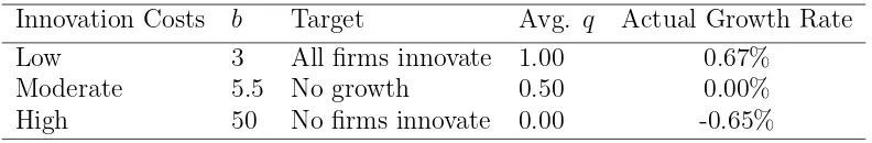
Table 2: Innovation Cost Calibrations
Innovation Costs b Target Avg. q Actual Growth Rate
Low 3 All firms innovate 1.00 0.67%
Moderate 5.5 No growth 0.50 0.00%
High 50 No firms innovate 0.00 -0.65%
cost economy, and a high cost economy. The functional form for innovation costs is
Hebq as in Atkeson and Burstien (2010). I set H = .001 to pin down the level of
costs and then calibrate the parameter b, to generate positive growth, zero growth,
and negative growth environments.18 The innovation costs are calibrated using a
baseline 20% tax rate. The lowest cost innovation environment is calibrated such
that all firms in the formal sector choose to innovate. I use the highest cost that
achieves this criteria. Further decreases in the costs of innovation marginally increase
growth but only through more firms switching to the formal sector. Likewise, in the
high cost environment, I find the lowest cost in which no firm decides to innovate.
Further increases in cost decrease growth, but only on the margin of sector choice.
Table 2 outlines the cost structures and growth rates used in the simulations.
Table 3 serves as a reference to the variables in the model, and Table 4 reports
specific parameter values use in the simulations. All of the simulations report results
for the first period in which firms operate, after making their sector choice. The
elasticity of substitution,ρ, is set to 5 as in Atkeson and Burstien (2010). While this
value is fairly standard, Hseih and Klenow (2009) discuss how even greater values
than ρ = 5 may be appropriate.19 Section 4.4 investigates the robustness of the
results to alternative values of ρ.
18Because the only source of growth in the model is increases in TFP, the maximum growth rate
is determined by the parameter ∆z.
Table 3: Variables of the Model
Variable Definition Variable Definition
ρ Elasticity of substitution c(q) Cost function for innovation
δ Probability of exit qit Probability of successful innovation
τ Tax rate on profits z¯t Spillover to informal sector
M Number of firms Γ Distribution of z0
wt Wage rate β Discount rate of firms
ˆ
zt Formal cut-off ∆z Step-size of innovation
L Labor Supply µ Probability of detection
Table 4: Parameter Values
Variable Value Source
ρ 5 Atkeson and Burstein (2010)
∆z 0.027 Brandt et al. (2012)
τ Varies World Development Index 2012
δ 0.10 Standard
β 0.96 Standard
M 10000 Scale parameter
L 100000 Scale parameter
Γ Uniform distribution See note below
qit Endogenously determined
wt Endogenously determined
The model is calibrated so that each time period corresponds to a year. Firms
anticipate a 10% chance of exit each year. I calibrate the step-size of innovation,
∆z, to correspond to 2.7% growth in TFP for the mean firm in the initial draw.
This estimate comes from Brandt et al. (2012) who estimate the average TFP
growth of manufacturing firms in China to be 2.7%. The implied discount rate, β,
the exogenous death rate, δ, and the step-size of innovation meet the parameter
[image:21.612.135.479.290.457.2]these parameter restrictions are not met, firms would be able to innovate faster than
future variable profits are discounted.
The productivity spillover is calibrated using Nataraj (2011).20 It reports mean
TFP for both the formal and informal sectors. Using these means and an estimate of
the variance, I generate a normal distribution to fit the distribution of log TFP that
she reports. I then calibrate the spillover such that the σ percentile of the formal
sector generates the mean TFP for the informal sector. I estimate that σ = 48.8,
that is, the 48.8th percentile of the formal sector matches the mean in the informal
sector. The value of ¯ztin the model is calculated as the TFP of the 48.8th percentile
of firms operating in the formal sector in time period t.
The initial distribution for z is drawn from a uniform distribution centered on
z = 0. As noted in the introduction, this does not translate into productivity being
uniformly distributed. Observed productivity in the model is ez/(ρ−1), so that the
distribution of productivity is exponentially distributed.21 Importantly, this
distri-bution shares many of the same characteristics of the Pareto distridistri-bution, mainly the
concentration of firms at the lower tail. Further discussion of the initial distribution
of firms is left for Section 5.
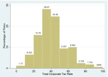
The range of taxes on profits is informed by data from the World Bank’s World
Development Indicators for 2012. Specifically, it reports the “Total Tax Rate,” which
is the total tax rate that firms pay as a percentage of their profits. It includes taxes
on profits, labor taxes, and other taxes like property and municipal taxes. For a
vast majority of countries, these taxes range from 10% to 70% of profits. Figure 1
20Her data is for pre-reform India in 1989, but it is the only data set I am aware of containing
TFP estimates for both formal and informal firms. Hsieh and Klenow (2010) report the distribution of plant size for both informal and formal firms in India, but do not provide firm-level productivity figures.
21This assumption is no different that assuming an exponential distribution for the initial
illustrates the range of tax rates and growth rates for a randomly selected subset of
countries included in the data. There are, however, several outliers that have tax
rates beyond 100%. These outliers seem to be driven by high “Other Tax Rates,”
likely reflecting political shocks that are beyond the scope of the current project (like
[image:23.612.127.488.233.491.2]one-time taxes on property).
Figure 1: Total Tax Rates (% of Firm Profits)
Source: World Development Indicators 2012. The histogram includes 171 countries that have available data on total tax rates as a percentage of firm profits. Countries with total tax rates above 100% are excluded.
In addition, the tax rate in the model should be understood to include corruption.
It is not quite clear whether this inclusion should raise or lower the actual tax rate
faced by formal sector firms. The 2005 World Bank Development report indicates
than formal sector firms. On the other hand, the incidence of paying bribes in
the informal sector was only about 50% of that in the formal sector. Given these
ambiguous factors, as well as the broad range of bribes and corruption documented
in Olken and Pande (2012), I take a conservative approach and suggest that the
presence of corruption may add from -5% to 5% (relative to the informal sector) to
the range of taxes in the formal sector. In totality, I look at tax rates (τ) from 5%
to 75% in the formal sector.
Finally,qis endogenously determined since firms choose the likelihood with which
their research and development is successful. However, in Atkeson and Burstein
(2010) the value of q is calibrated for large firms in order to keep the dynamics of
those firms constant through time. In the current model, all firms make decisions
regarding how much to innovate. In both the high cost and low cost environments,
there is little to no heterogeneity in firms’ choice of q, but there is considerable
heterogeneity in the costs associated with innovation.
4
Results
The results are presented in four sections. The first section explores and develops
intuition for how the model operates. Specifically, it illustrates the distribution of
productivity resulting from firm sectoral choice and the spillover of technology. The
next set of results investigates how innovation affects the sectoral decision of firms.
It clearly shows that changes in tax rates have significant impacts on the size of the
informal sector. The third section looks at the aggregate effect of the changes in
sector choice. I find that changes in the tax rate have significant impacts on the size
of the informal economy and TFP growth. The final section tests the robustness of
are fort = 1, the first period in which firms realize their sector decisions and operate
in their chosen sector. Therefore, changes in innovation costs and tax rates should
be seen as changing this initial sector decision and not as a reallocation within the
first period.
4.1
Developing Intuition
It is important to develop some intuition for how firms enter each sector. Firms that
decide to enter the informal sector forgo the ability to innovate and instead receive
a productivity spillover from the formal sector, ¯zt. Figure 2 illustrates how this
assumption operates. It orders firms from lowest productivity to highest productivity
after firms have made their sectoral choice. It clearly illustrates the division of firms
into each sector and underscores why it is important to model the dynamic decisions
of firms. The left-hand side of Figure 2 is populated by lower productivity firms that
operate in the formal sector. These firms anticipate the gains from innovation to
exceed the lost profits from taxation. Since these firms produce a unique intermediate
good, they are not driven out of the market. A large swath of the economy operates
informally with the fixed (within each period) productivity ¯z. The right-hand side
of Figure 2 is populated by high productivity formal sector firms. It is still the case,
as in Rauch (1991), that a firm with a higher initial productivity parameter,zi0, will
tend to enter the formal sector.
The model generates a large mass of firms at the lower end of the distribution
of productivity, as can be seen in Figure 3. Since firms hire labor proportionally
to ez, Figure 3 also implicitly determines the distribution of firm size. For now,
it is important to note that there will be a large number of relatively small firms.
operating at roughly 13 the productivity level of the most productive firms. Further
discussion of alternative distributions for initial productivity and the desirability of
[image:26.612.123.489.209.501.2]this distribution is left for Section 5.
Figure 2: Firm Productivity
The figure is generated using 10,000 firms that face a 20% tax rate on profits in the formal sector. Innovation costs are moderate (b= 5.5) andρ= 5. Note that observed productivity in the economy is actuallyeρ−1z , which means that z = (ρ−1)log(observed TFP). In the figure above, 61.3% of
Figure 3: Distribution of Firm TFP
4.2
Informality and Innovation
In order to discuss impacts on aggregate variables, it is first necessary to illustrate the
role that innovation has on firm sector choice. If innovation does not have a significant
impact on firm choice, the complexity added through integrating innovation within
a model of monopolistic competition is likely not an improvement over earlier static
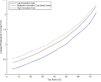
models of sector choice. Figure 4 plots the cut-off value, ˆz, for firms to enter the
[image:28.612.124.479.309.598.2]formal sector.
Figure 4: Cut-off Value of Initial Productivity for Entry into the Formal Sector
The effect of taxation on the productivity cut-off is illustrated for the three
differ-ent cost levels of innovation as described in Table 2. The more expensive innovation
is, the less incentive there is to operate formally. The value of ˆz with high innovation
costs is always higher than ˆz under lower innovation costs. Since ˆz represents the
lowest value of productivity that firms would need to enter the formal sector, lower
values of ˆz correspond to additional firms entering the formal sector. Lowering the
cost of innovation raises the valuation of firms in the formal sector who can pursue
[image:29.612.120.489.320.617.2]innovation to increase their future productivity and profits.
Figure 5: Percentage of Firms Operating in the Formal Sector
These results are corroborated in Figure 5. Reducing the cost of innovation
in-creases formal sector participation at every tax rate. More firms opt to improve their
production processes rather than simply produce using the productivity spillover
from the formal sector. These changes in sector size over the different tax rates are
quite sizable. In the moderate cost innovation environment the formal sector is
re-duced by 82% across all tax rates considered (5% to 75%). Smaller changes in the
tax rate have important effects too. For instance, an economy with a 50% tax rate
would see a 17.5% increase in the size of the formal sector from cutting taxes by 10%
or a 20.9% increase by raising them 10%. Notice that at higher levels ofτ, firms opt
into the informal sector at an increasing marginal rate.
The process above is augmented by the gradual increase in the size of the spillover
as firms migrate to the informal sector. Suppose that taxes are increased just enough
to persuade one additional firm to be informal rather than formal. This marginal
change affects the size of the spillover from the formal sector. As the lowest
produc-tivity firm in the formal sector switches to the informal sector, it raises the average
productivity in the formal sector, increasing the spillover, ¯zt, to the informal sector.
This process is illustrated in Figure 6.
An immediate effect of the technology spillover is that higher costs of innovation
lead to higher productivity levels in the informal sector. This feature has two intuitive
interpretations. First, it reflects the fact that in economies with higher costs of
innovation, more productive entrepreneurs may eschew innovation and instead evade
taxes in the informal sector. Second, it also implies that higher innovation costs lead
to a smaller dispersion of productivity. While it may be counter-intuitive that the
informal sector ought to be more advanced in a society with higher innovation costs,
this effect is temporary. Firms in the low cost economy innovate with q = 1, while
Figure 6: Productivity Spillover to Informal Firms
of q correspond to greater innovation and TFP growth, the lower innovation costs
today, the higher the productivity of formal sector firms in the future.
4.3
Informality and Aggregate Effects
As the tax rate increases, the ratio of output in the informal sector to total output
increases, as can be seen in Figure 7. In absolute terms, however, the amount of
output that is produced in the informal sector is relatively small when compared
to data on the size of informal sectors in developing counties, as seen in Table 1.
Informal firms, with their smaller productivity levels of ¯z, operate on a smaller scale
than their formal sector counterparts. They are, however, more numerous under
all of the specifications I evaluate. Further discussion of this result is also left for
Section 5.
In certain innovation environments, the tax rate changes the rate of TFP growth.
This process is plotted in Figure 8. As taxes increase, the returns to innovating
in the formal sector decrease. This entails both lower innovation rates, as well as
lower formal sector participation as documented previously. I find that TFP growth
decreases by .07% for a 10% tax increase from 50% to 60%. This affect occurs despite
the fact that the size of the spillover to the informal sector mechanically increases as
the tax rate increases. For a fixed productivity spillover, the decrease in TFP growth
would be substantially larger.
In both the high and low cost environments, the costs of innovation dominate
changes in the tax rate such that the innovation rate does not change, and hence
TFP growth rate does not change. In those settings, as τ increases, firms flee the
formal sector, leaving fewer innovators, as seen in Figure 5. This process also drives
Figure 7: Percentage of Output Produced in the Informal Sector
any accompanying change in innovation rates among formal sector firms leads to no
change in TFP growth. Firms in the real world are not likely at either of those bounds
and do change their innovation activities in response to changes in corporate tax
rates. Recall that in these extreme environments firms invest in research sufficiently
to ensure success or make failure a certainty. Given that real world innovation does
[image:34.612.143.470.268.546.2]not likely follow this model, I focus my analysis on the moderate costs environment.
Figure 8: Growth in Aggregate TFP
4.4
Robustness
Below I investigate the effects of changing the value ofρ in the simulations. The
pa-rameter ρgoverns the substitutability of different intermediate goods in the
produc-tion of the final good. As ρ increases, the substitutability between goods increases,
decreasing market power and the incentives for firms to innovate in the formal
sec-tor. This result is illustrated in Figure 9. Notice that the percentage of total output
produced in the informal sector increases withρ. In the case of ρ= 7, the informal
economy has a much larger impact, constituting 11.5% to 20.2% of the economy.
Changes in ρ also affect TFP growth, as can be seen in Figure 10. The case of
ρ = 3 is unique. In that case, changes in the tax rate are dominated by incentives
to innovate. Mainly that given the costs, lowering ρ increases the profitability of
innovating, as static profits are proportional to productivity in the model. This is a
very similar set of circumstances that explained why TFP growth did not vary for
ρ = 5 (base case) in the high and low cost innovation environments. Raising the
value of ρ lowers the level of TFP growth as firms are less profitable because their
market power diminishes. Overall, changes in the value ofρ have predictable effects
resulting from static profits decreasing asρincreases. This translates into decreasing
the profitability of innovation.
The sensitivity of the model to changes in the elasticity of substitution should
not be surprising. In fact, it reflects an unresolved question in the literature on
informality: do formal and informal firms compete? According to recent work by La
Porta and Sheifer (2014) firms do not compete across sectors. On the other hand,
data from the World Bank Enterprise surveys suggests that many formal firms do in
fact compete. It could also be that there is a strong complementarity between sectors
Figure 9: Percent of Total Output Produced by Informal Firms
choice of ρ = 5 seems like prudent choice given its previous use in the literature.
Modeling firms as competing in monopolistic competition seems to be a compromise
[image:37.612.135.471.203.481.2]between alternatives in the literature that allows reasonable levels of competition.
Figure 10: TFP Growth across Values of ρ
Innovation costs are as referenced in Table 2. The tax rate corresponds to τ in the model. See caption on Figure 9 for an explanation whyρ= 3 does not appear for levels ofτ≥.65.
5
Discussion
Below, I focus on three areas of particular concern/interest: the parameterization
to the informal sector, and the assumption of firms making a single entry decision.
These areas seem to be responsible for both the desirable qualities of the model, as
well as some of its shortcomings.
The parameterization of initial productivity in the model is a particularly
nebu-lous issue. In most developing countries, the distribution of productivity generates
a firm-size distribution with a large number of small firms as documented in Tybout
(2000). In the current application, firm-size is linked to firm productivity such that
less productive firms are also smaller. In this sense, the current parameterization
cap-tures the ubiquity of small firms that is documented by Tybout (2000). Choosing a
realistic initial distribution hinges on two competing concerns. First, the dispersion
of productivity is responsible for determining how relevant the informal sector is.
A smaller dispersion of productivity implies that firms in the informal sector will
produce a greater percentage of total output. Drawing the initial productivity from
a narrower range ofz would increase the significance of informal firms.
On the other hand, the desire to calibrate the distribution to match data regarding
the size of informal economies must be tempered by a realistic assessment of how
productive formal sector firms are compared to informal sector firms. As the 2013
World Development Report points out, few countries collect reliable data on the
informal sector, and there are few reliable estimates of the true ratio of productivity
between the sectors. Hsieh and Klenow (2009) establish a lower bound by reporting
that the ratio log TFP for the 90th percentile to the 10th percentile is 5.0 for India
and 4.9 for China. These numbers represent a lower bound since both small and
informal firms are excluded from their data sources.
As a means for comparison, in a simulation with moderate innovation costs and
a tax rate of 20%, the ratio of the highest productivity firm to the productivity
TFP to lowest TFP is 4.17. Especially with regard to the second statistic (which
is most similar to that of Hseih and Klenow (2009)), the initial productivity draw
seems entirely plausible. The first statistic is more difficult to compare since, to my
knowledge, there is no analog in the literature.22 The World Bank Enterprise Survey
(WBES) has collected data on both formal and informal sector firms, but those data
sets are usually collected in different years and do not yield comparable measures of
productivity across formal and informal firms.
It is important to note that based on the data in Nataraj (2011), the model
incorporates the overlap in productivity between the formal and informal sector.
This element is not seen in earlier models of sectoral choice. In those models, such as
Rauch (1991), there is a strict dualism where firms in the informal sector are always
less productive than the least productive formal firms.
Closely related to the choice of initial distribution of firm productivity is how
productivity spills over to the informal sector. Decreasing the size of the spillover,
for instance, by endowing firms in the informal sector with the lowest quartile of
productivity in the formal sector, would decrease the incentives to switch sectors
when taxes increase. At the same time, such a change would increase the ratio of
productivities between the sectors by lowering productivity in the informal sector.
Ultimately, the spillover used in the model is the only one that can be readily justified
given the available data.
A larger question: does such a spillover make sense? The nature of the spillover is
intended to capture the fact that firms in the informal sector tend to adopt changes
investing substantially less in innovation. In this sense, their productivity improves
22This measure is tied to the size of the spillover from the formal to informal sector. The
over time, but is not at the technological frontier. For instance, evidence from the
World Enterprise Survey indicates that smaller (highly correlated with informal)
firms are less likely to utilize e-mail. This indicates that some firms choose to adopt
new technologies that are already commonplace in the formal sector. Informal sector
firms did not invent e-mail or revolutionize its applications, but adopt its usage to
improve their productivity when they see its widespread usage in the formal sector.
The answer to how realistic the specification of the spillover is, ultimately hinges
on country-specific context. For instance, informal production in some countries
may resemble relatively simple home production. This production may occur in
rural areas that are not in close proximity to dense manufacturing areas. On the
other hand, in places like India, some data indicates that there is a complementarity
between production in the formal and informal sectors. Sundaram et al. (2012)
document a strong positive correlation between factor movements in the formal sector
and informal sector. They conclude that there is likely a strong complementarity
between the sectors. In this case, spillovers may be larger than currently specified in
the model.
Part of the complementarity that Sundaram et al. (2012) document is the ability
of the informal sector to absorb excess labor and provide employment for workers
who cannot find work in the formal sector. One reason the model does not accurately
reflect the size of informal economies is that labor is the sole factor of production.
Informal firms tend to be more labor intensive, while formal sector firms tend to be
more capital intensive. Introducing a complementarity between the two sectors may
increase the size of the informal sector so that it better reflects the available data.
Additionally, as noted in Section 4.4, a higher level of substitutability between the
formal and informal sector (i.e. higherρ) could also explain the size of the informal
Finally, it is worth discussing the validity of looking at firms’ sector decisions,
assuming that they stay in that sector rather than switching in a later period. While
this assumption is made principally to isolate the role of innovation on firms’
de-cisions, there are reasons to suggest that there are barriers to switching sectors.
Nataraj (2011) reports that few firms in India switch from formal to informal
de-spite having fewer employees than is necessary to be required to register as a formal
firm. Additionally, barring a bad series of innovation shocks, the incentives for firms
that reach high enough productivity levels to have them opt into the formal sector,
would still seek to stay there. On the informal side, there is substantial data to
sug-gest that there are large barriers to entry for the formal sector that are not explicitly
modeled here. These costs would be incurred in addition to a higher tax rate, and
they may deter firms from switching sectors.
6
Conclusion
This paper investigates how firms react to changes in government policy and
de-termine whether to operate formally or informally. Not only are firms’ decisions
shown to be significantly affected by taxes and innovation costs, but their sectoral
choices also have important impacts on aggregate variables such as TFP growth.
Considering the importance of TFP in determining cross country income differences,
understanding how firms’ dynamic sectoral decisions are influenced by taxation is a
positive step in understanding the process of development.
By modeling how firms react to changes in tax rates, make innovation decisions,
and decide which sector to operate in, I am able to generate relevant policy
impli-cations. Specifically, governments limit TFP growth through taxation by pushing
firms. Secondly, institutions that lower the costs of innovation are better for
entic-ing firms to operate formally. This work improves on previous understandentic-ing of the
informal sector by explicitly modeling the dynamic decision making process of firms.
Ultimately, it underscores the role of government policy in shaping the incentives
of individuals and firms. Given the right incentives, these individuals and firms are
References
[1] Atkeson, A., and A. Burstein (2010). “Innovation, Firm Dynamics, and Inter-national Trade.” Journal of Political Economy, 118(3), 433-484.
[2] Auriol, E., and M. Warlters (2005). “Taxation Base in Developing Countries.” Journal of Public Economics, 89(4), 625-646.
[3] Brandt, L., J. Van Biesenbroeck, and Y. Zhang (2012). “Creative Accounting or Creative Destruction? Firm-level Productivity Growth in Chinese Manufac-turing.” Journal of Development Economics, 97(2), 339-351.
[4] Dabla-Norris, E., M. Gradstein, and G. Inchauste (2008). “What Causes Firms to Hide Output? The Determinants of Informality.” Journal of Development Economics, 85, 1-27.
[5] De Soto, H. (1989). The Other Path: The Invisible Revolution in the Third
World, New York: Harper and Row.
[6] De Soto, H. (2000). The Mystery of Capital: Why Capitalism Triumphs in the
West and Fails Everywhere Else, New York: Basic Books.
[7] Goldberg, P.K., and N. Pavcnik (2003). “The Response of the Informal Sector to Trade Liberalization.” Journal of Development Economics, 72, 463-496.
[8] Grossman, G.M., and E. Helpman (1991). “Quality Ladders in the Theory of Growth.” Review of Economic Studies, 58(1), 43-61.
[9] Hall, R.E., and C.I. Jones (1999). “Why Do Some Countries Produce So Much More Output Per Worker Than Others?” Quarterly Journal of Economics, 114(1), 83-116.
[10] Henley, A., G.R. Arabsheibani, and F.G. Carneiro (2006). “On Defining and Measuring the Informal Sector.” IZA Discussion Papers, No. 2473.
[11] Hsieh, C., and P.J. Klenow (2009). “Misallocation and Manufacturing TFP in China and India.” Quarterly Journal of Economics, 124(4), 1403-1448.
[12] Hsieh, C. and P.J. Klenow (2010). “Development Accounting.” American Eco-nomic Journal: MacroecoEco-nomics, 2(1), 207-223.
[13] Judd, K.L. (1992). Numerical Methods in Economics, Cambridge, Mass.: MIT
[14] Kanbur, R. (2009). “Conceptualising Informality: Regulations and Enforce-ment.” Indian Journal of Labor Economics, 52(1), 33-42.
[15] La Porta, R. and A. Shleifer (2014). “Informality and Development.” Journal of Economic Literature, 28(3), 109-126.
[16] Levy, S. (2008). Good Intentions, Bad Outcomes: Social Policy, Informality,
and Economic Growth in Mexico, Brookings Institution Press.
[17] Loayza, N.V. (1996). “The Economics of the Informal Sector: A Simple Model and Some Empirical Evidence from Latin America.” Carnegie-Rochester Con-ference Series on Public Policy, 45, 129-162.
[18] Lucas, R.E. (1978). “On the Size Distribution of Business Firms.” Bell Journal of Economics, 9(2), 508-523.
[19] Luttmer, E.G.J. (2007). “Selection, Growth, and the Size Distribution of Firms.” Quarterly Journal of Economics, 122, 1103-1144.
[20] Melitz, M.J. (2003). “The Impact of Trade on Intra-Industry Reallocations and Aggregate Industry Productivity.” Econometrica, 71, 1695-1725.
[21] Nataraj, S. (2011). “The Impact of Trade Liberalization on Productivity: Ev-idence from India’s Formal and Informal Manufacturing Sectors.” Journal of International Economics, 85(2), 292-301.
[22] Olken, B.A., and R. Pande (2012). “Corruption in Developing Countries.” An-nual Review of Economics, 4(1), 479-509.
[23] Olson, M., Jr. (1982). The Rise and Decline of Nations, Economic Growth,
Stagflation, and Social Rigidities, New Haven, Conn.: Yale University Press.
[24] Rauch, J.E. (1991). “Modeling the Informal Sector Formally.” Journal of Eco-nomic Development, 35, 33-47.
[25] Rosenzweig, M.R., and H.P. Binswanger (1993). “Wealth, Weather Risk, and the Composition and Profitability of Agricultural Investments.” The Economic Journal, 103(416), 56-78.
[27] Sundaram, A., R.N. Ahsan, and D. Mitra (2012). “Complementarity between Formal and Informal Manufacturing in India,” in J. Bhagwati and A.
Pana-gariya (Eds.) Reforms and Economic Transformation in India, Oxford
Univer-sity Press.
[28] Thomas, J.J. (1992).Informal Economic Activity, Ann Arbor, Mich.: University
of Michigan Press.
Appendix A
This section outlines the derivation, calculation, and assumptions for calculating aggregate output growth. Let the aggregate growth rate be designated
gY =
Yt+1−Yt
Yt
. (21)
Substituting (19) in for Yt and its equivalent for Yt+1, yields (20). Recall that
Zt=
X
i
ezit, (22)
for all firms, both formal and informal. Aggregate productivity can be split into formal and informal sectors as
Zt = zmax
X
ˆ
z
ezit +
ˆ
z
X
zmin
ez¯t, (23)
with a slight abuse of notation with the indexing on the sums. The formal sector is composed of all firms with draws of z ∈ [ˆz, zmax]. Recall that ¯zt is equal to the σ
percentile of productivity in the formal sector. Let ω be the number of firms that
participate in the formal sector. Similarly, letξ be the number of firms that operate
in the informal sector. Aggregate TFP at time t then is
Zt= zmax
X
ˆ
z
ezit+ξez¯t (24)
A similar expression can be derived for the expected value ofZt+1. Given the process
of innovation outlined in Section 2.3, firm’s expected productivity in the formal sector is
Etezit+1 =qitezit+∆z+ (1−qit)ezit−∆z. (25)
Thus, EtZt+1 can be written similarly to (24):
EtZt+1 =
zmax
X
ˆ
z
Etezit+1+ξEte¯zit+1, (26)
subject to (25). Notice that this result utilizes the fact that firms make a decision to enter a given sector under assumption that they will stay in that sector. Under this
assumption, the distribution of firms into each sector, mainly the parameters ω and
ξ are fixed. Combining equations (20), (24), and (26) allows for the calculation of
expected output growth. Expected output growth is a function of the distribution of firms productivity,zt, the cut-off value ˆz that determinesω and ξ, and firms’ choices