A new financial metric for the art market

Munich Personal RePEc Archive

A new financial metric for the art market

Charlin, Ventura and Cifuentes, Arturo

V.C. CONSULTANTS, Santiago, CHILE, Financial Regulation

Center Faculty of Economics and Business University of Chile

Santiago, CHILE

23 September 2013

Online at

https://mpra.ub.uni-muenchen.de/57139/

A

N

EW

F

INANCIAL

M

ETRIC FOR THE

A

RT

M

ARKET

(Working Paper, April 2014)

Ventura Charlin (1)

V.C. Consultants

Los Leones 1300, Suite 1202

Santiago, CHILE

e-mail: ventcusa@gmail.com

Arturo Cifuentes

Financial Regulation Center (CREM)

Faculty of Economics and Business

University of Chile

Santiago, CHILE

e-mail: arturo.cifuentes@fen.uchile.cl

(1) author to whom all correspondence regarding this paper should be addressed. Comments

Abstract

This paper introduces a new financial metric for the art market. The metric, which we call

Artistic Power Value (APV), is based on the price per unit of area (dollars per square

centimeter) and is applicable to two-dimensional art objects such as paintings. In addition to

its intuitive appeal and ease of computation, this metric has several advantages from the investor’s viewpoint. It makes it easy to: (i) estimate price ranges for different artists; (ii) perform comparisons among them; (iii) follow the evolution of the artists’ creativity cycle

overtime; and (iiii) compare, for a single artist, paintings with different subjects or different

geometric properties. Additionally, the APV facilitates the process of estimating total

returns. Finally, due to its transparency, the APV can be used to design derivatives-like

instruments that can appeal to both, investors and speculators. Several examples validate

this metric and demonstrate its usefulness.

Keywords Art markets Hedonic models Paintings Auction prices

JEL Classification C18 D44 G11 G12 Z10

Note:The authors would like to thank Robert Yang whose technical expertise was

Background

In the last thirty years, the art market –and more precisely, the market for paintings−has

received an increasing amount of attention from economists, financial analysts, and investors.

They have brought to this field many quantitative techniques already employed in more

conventional markets. Not surprisingly, one topic that has received a great deal of attention

is returns, specifically, how to compute returns for the art market. This is a challenging task

not only because this market is still rather illiquid, at least compared with equities and bonds,

but also because of its heterogeneity: every painting is essentially a unique object.

Several authors have employed hedonic pricing models (HPMs) to estimate returns

(e.g., Chanel et al., 1994, 1996; de la Barre et al., 1994; Edwards 2004; Renneboog and

Spaenjers 2013). Such models are suitable to manage product variety and can use all the

available data. Their drawback, however, is that their application is limited by the

explicatory power of the variables selected and sometimes it is difficult to fit a good model to

the data (the academic literature frequently reports models with values of R2 around 60% or

below). Moreover, if the data are sparse (a common situation, especially for individual

artists) the application of HPMs might not be possible (Galbraith and Hodgson 2012). An

additional disadvantage of HPMs is the lack of stability that often affects the computation of

the hedonic regression coefficients, coupled with the lack of reliability −not to mention the

not-so-straightforward interpretation− of the time dummies (Collins et al., 2007). Finally,

price indices based on the time-dummies do not satisfy the monotonicity condition --an

essential requirement for any price index (Fisher, 1922; Melser, 2005). This is a critical issue

for violation of this condition might lead to spurious returns, a fact that the cultural

economics community has not yet acknowledged.

A second alternative to estimate returns is to rely on repeat sales regressions (e.g.,

Anderson 1974; Baumol 1986; and Goetzmann 1993). While this approach has the

advantage of using price data referring to the same object it has two disadvantages: a

potential selection bias and the fact that it only employs a small subset of the available

information. Ginsburgh et al. (2006) provide an excellent discussion on the merits of each

approach plus a fairly complete literature review. Mei and Moses (2002); Renneboog and

Spaenjers (2011); Higgs and Worthington (2005); Agnello and Pierce (1996); and artnet

Analytics (2012) have dealt with the construction of art indices based on the two

The question of which approach is better to estimate returns still remains open. This

issue is far more vexing than it appears. Superficially, it might be interpreted as a choice

between two methods that lead to the same answer based on computational ease. However,

there is no assurance that this is indeed the case. In fact, they might lead to different answers

and it is not always clear which answer is the right one. Ashenfelter and Graddy (2003) have

stated this point more forcefully: ‘The hedonic index gives a real return of about 4 percent, while the repeat-sales index results in a real return of about 9 percent! Which is correct?’

Previous researchers have also focused on other topics. Just to name a few: Galenson

(1999); Galenson (2000); Galenson (2001); Galenson and Weinberg (2000); and Ginsburgh

and Weyers (2006) have looked at the creativity cycle of several artists (that is, the age at

which they produced their best work). Renneboog and Van Houte (2002); Worthington and

Higgs (2004); Renneboog and Spaenjers (2011); and Pesando (1993) have compared the

returns of certain segments of the art market vis-à-vis more conventional investments. Coate

and Fry (2012) and Ekelund et al. (2000) have investigated the death-effect in the price of

paintings. Edwards (2004) and Campos and Barbosa (2009) have looked at the performance

of Latin American painters. Scorcu and Zanola (2011) used a hedonic model approach to

study Picasso’s paintings, while Higgs and Forster (2013) investigated whether paintings

which conformed to the golden mean commanded a price premium. And, Sproule and

Valsan (2006) questioned the accuracy of hedonic models compared with the appraisals of

experts.

Other issues that have been investigated, some of them still with inconclusive answers,

are: whether the lack of signature affects the auction price of a painting; the importance of the

auction house (in essence, Sotheby’s or Christie’s versus lesser known auction houses);

whether masterpieces tend to underperform when compared to less expensive paintings; the

correlation between the art market and the major equity and fixed income indices; whether an

artist can be described, based on its creativity-cycle curve, as conceptual (early bloomer) or

experimentalist (late bloomer); as well as the relationship between, withdrawing a painting

from an auction, and its future sale price. All these analyses have relied on statistical and

modeling techniques commonly used in financial and economic analysis.

In summary, although a great deal has been learned about the financial aspects of the

art market in recent years, much needs to be understood, especially, from the investor’s

mentioned. In addition, we want to shift the focus towards the investor’s viewpoint and

move away from the purely econometric models which, even though are interesting from an

academic angle, offer little guidance to somebody concerned with pricing issues. Thus, our

goal is twofold: (i) to provide a new tool to enrich the analysts’ toolbox; and (ii) to facilitate the investors’ decision-making process by making it easier to assess the merits of a painting using some simple quantitative analyses.

We should note that the application of HPMs and repeat sales regression models has so

far focused, mainly, on estimating market returns aimed at building indices. Although these

indices can be useful for performing econometric analyses and describing market tendencies,

in general, they are less useful for investors. The chief reason is that investors are concerned

with actual or realized returns (that is, total returns) instead of returns based on an ideal

painting whose characteristics do not change over time (which is the case of time-dummies

based returns). To put the point more forcefully: an investor has little use for an index that

controls for quality and paintings’ characteristics. In fact, the investor wants information that actually captures these features as well as supply-demand dynamics. The metric introduced

herein (a point we discuss in more detail later) captures exactly that.

A New Financial Metric

Paintings, notwithstanding their artistic qualities, are essentially two-dimensional

objects that can command −sometimes− hefty prices. Based on this consideration, it makes

sense to express the value of a painting not using its price but rather a price per unit of area

(in this study, dollars per square centimeter). We call this figure of merit Artistic Power

Value or APV. By normalizing the price, the APV metric intends to offer the investor a

financial yardstick that goes beyond the price, while not attempting to control for the

specifics of the painting beyond its area.

The intuitive appeal of this metric is obvious: simplicity, ease of computation,

transparency, and straightforwardness. In fact, there is already a well-established precedent

for this approach. For example, prices of other two-dimensional assets, such as raw land, are

frequently quoted this way (e.g. dollars per acre, or euros per hectare). The same approach is

sometimes used to quote prices of antique rugs.

More recently, many artisans, print makers, digital printing firms, and poster designers

have started to quote price estimates using this same concept. Moreover, considering that the

two-dimensional objects is often estimated on a per-unit-of-area basis, the idea of extending

the same notion to express the value of the final product is not far-fetched.

Finally, the rationale for using the APV metric is not to negate the individuality of each

painting or to trivialize the artistic process. It is really an attempt to synthetize in one

parameter the financial value of a painting (or artists or body of work) with the goal of

making comparisons easier. Additionally, many APV-based computations (a point treated in

more detail in the subsequent section) can offer useful guidance for pricing purposes.

Alternatively, we can think of the APV as an attempt to find a common factor to

compare and contrast the economic value of otherwise dissimilar art objects. If we accept the

thesis that two paintings −even if they are done by the same artist and depict the same theme−

are not only different but also unique, it is not possible to make a straight price-wise

comparison. However, the APV metric, by virtue of removing the size-dependency, helps to

make this comparison possible: in a sense the APV plays the role of unitary price.

The Data

Three data sets are employed in this study:

a. Data set A consists of 1,820 observations of Pierre-Auguste Renoir’s paintings

auction prices and their characteristics covering the period [March 1985; February 2013].

The database was built based on information provided by the artnet database

(www.artnet.com).

b. Data set B consists of 441 observations of Henri Matisse’s paintings auction

prices and their characteristics covering the period [May 1960; November 2012]. The

database was built based on information provided by the artnet database (www.artnet.com)

and was supplemented by additional auction data from the Blouin Artinfo website

(www.artinfo.com).

c. Finally, data set C consists of 2,115 observations of paintings covering the

period [March 1985; February 2013]. This data set gathers information from six artists

(Alfred Sisley, Camille Pissarro, Claude Monet, Odilon Redon, Paul Gauguin, and Paul

Signac) and was based on auction information provided by the artnet database.

All prices were adjusted to January-2010 U.S. dollars (using the U.S. CPI index) and

selling price was below US$ 10,000 or the APV was less than 1 US$/cm2 were eliminated.

Sotheby’s and Christie’s dominate the data sets, as together they account for 86% of the

sales.

The selection of artists was somewhat arbitrary. The chief consideration was to

effectively examine the merits of the APV metric without regard to the qualities of the

painters selected. Renoir was an ideal choice because of the high number of observations

available, which were distributed over a long period of time, and without time-gaps. This

situation facilitates the comparison between the APV metric and the HPMs (which require

many data points to be built). Matisse data had the advantage of being distributed over a

longer time span, but included less observations, and had a few time-gaps. Data set C,

despite its strong impressionist flavor, was not aimed at capturing in full the characteristics of

the impressionist movement; it represents a group of painters who happened to live roughly at

the same time and for which there were enough observations to make certain computations

feasible. Nevertheless, and simply for convenience, in what follows we refer to this group as

the Impressionists group. Renoir, despite his strong impressionist credentials was purposely

left out of data set C. Otherwise, he would have dominated the group, making it highly

correlated with data set A: an undesirable situation given the need to test the APV metric

under different scenarios.

In summary, the selection of artists was not done with the idea of deriving any specific

conclusion regarding these painters or the artistic tendencies they represented; the leading

consideration was to showcase the attributes and benefits of the APV metric.

Table 1 summarizes the key features of the three data sets. Table 2 describes in more

detail the characteristics of the painters in the Impressionist group (data set C). Notice that

the APV distribution is far from normal: the differences between the arithmetic mean

(average) values and the medians are manifest, with the means always higher than the

medians. Additionally, the values of the skewness and kurtosis reveal a strong positively

skewed distribution with fat tails. The Jarque-Bera (JB) statistic and its corresponding

p-value (close to 0.000 for each of the three data sets) indicate that the APV is not normally

distributed. These facts should serve as a warning against APV-based projections based on

normality assumptions. Finally, the relatively high values of the coefficient of variation for

several artists (Renoir and Matisse exhibit the most variability) are somehow evidence of

what experts already know: even masters are uneven producers and their paintings differ

consistent with the critics’ assessment of their merits, it is a topic we leave for others to

decide

Table 1. Description of the three data sets and key statistics

Data Set: A Data Set: B Data Set: C

Artist Pierre-Auguste Renoir Henri Matisse Impressionists group

Born–Died 1841–1919 1869–1954 NA

Number of Sales 1,820 441 2,121

Period of Sales Mar 1985–Feb 2013 May 1960–Nov 2012 Mar 1985–Feb 2013

Geometric Mean APV (US$/cm2) 399 356 312

Median APV (US$/cm2) 377 308 311

Average APV (US$/cm2) 646 803 537

Standard Deviation (US$/cm2) 1,331 1,332 786

Coefficient of Variation 2.06 1.66 1.46

Skewness 15.56 3.87 4.86

Kurtosis 344.06 19.83 31.87

Jarque-Bera 9,040,581.38 8,328.44 97,801.30

JB p-value 0.000 0.000 0.000

Table 2. Detailed characteristics and key statistics of the artists included in data set C

Artist Number of Sales

Born– Died

Average APV (US$/cm2)

Standard Deviation (US$/cm2)

Coeff. of Variation

Geometric Mean APV (US$/cm2)

Median APV (US$/cm2)

Alfred Sisley 343 1839–1899 389 282 0.73 311 313

Camille Pissarro 586 1839–1903 432 335 0.78 324 338

Claude Monet 586 1840–1926 760 999 1.31 422 411

Odilon Redon 193 1840–1916 167 156 0.93 109 118

Paul Gauguin 167 1848–1903 1,138 1,631 1.43 539 465

Applications of the APV Metric

This section is intended to demonstrate the usefulness of the APV metric with the help

of some examples.

Comparisons Among All Artists

The fact that the APV follows a highly non-normal distribution calls for comparisons to

be based on the median rather than the average value. To this end we employ the median

comparison test using the Price-Bonett variance estimation for medians (Price and Bonett

2001; Bonett and Price 2002), described in Wilcox’s (2005) review of methods for comparing

medians.

Table 3. Comparisons among the APV medians for all artists (1985-2012 sales only)

Median APV (diagonal) Difference between medians (off-diagonal)

(US$/cm2₎

Henri Matissea Paul Gauguin Claude Monet Pierre-Auguste Renoir Camille Pissarro Alfred Sisley Paul Signac Odilon Redon

Henri Matissea 513

Paul Gauguin NS 465

Claude Monet 102** NS 411

Pierre-Auguste Renoir 136*** 88* 34* 377

Camille Pissarro 175*** 127** 73*** 39*** 338

Alfred Sisley 200*** 152** 98*** 64*** 25* 313

Paul Signac 311*** 263*** 209*** 175*** 136*** 111*** 202

Odilon Redon 395*** 347*** 293*** 259*** 220*** 195*** 84*** 118

NOTE:a: Median calculated from sales between 1985-2012 only; NS: Not Significant; *p<.10; **p<0.05; ***p<0.01

Table 3 summarizes the results of such comparison. The median values for each artist

are shown along the diagonal with the values decreasing from top-left to bottom-right:

Matissse1 has the highest value (513 US$/cm2) while Redon the lowest (118 US$/cm2). The

remaining entries in the table can be interpreted, using matrix notation, as follows: the (i, j)

entry represents the median APV value of artist j minus the median APV value of artist i.

Hence, Pissarro’s median APV exceeds that of Signac by 136 US$/cm2

while there is no

significant difference between Gauguin and Matisse’s median APVs.

1

These calculations, trivial by all accounts, offer a convenient way to rank artists. They

also offer useful guidance for pricing purposes.

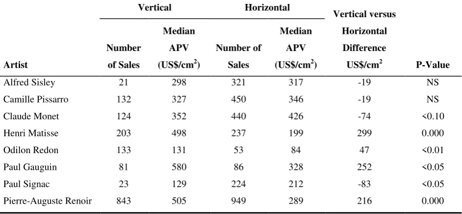
Vertical versus Horizontal Orientation for a Given Artist

Table 4. Comparisons of APV medians: vertical versus horizontal oriented paintings

for each artist

Artist

Vertical Horizontal

Vertical versus Horizontal Difference

US$/cm2 P-Value Number

of Sales

Median APV (US$/cm2)

Number of Sales

Median APV (US$/cm2)

Alfred Sisley 21 298 321 317 -19 NS Camille Pissarro 132 327 450 346 -19 NS Claude Monet 124 352 440 426 -74 <0.10 Henri Matisse 203 498 237 199 299 0.000 Odilon Redon 133 131 53 84 47 <0.01 Paul Gauguin 81 580 86 328 252 <0.05 Paul Signac 23 129 224 212 -83 <0.05 Pierre-Auguste Renoir 843 505 949 289 216 0.000

NOTE: Paintings with height=width are excluded from the table. NS: Not significant.

Certain painters, Modigliani for instance (not part of this study) decidedly preferred the

vertical orientation. Sisley and Signac, on the contrary, favored the horizontal orientation.

Table 4 compares, for all the artists considered here, the median APV as a function of the

orientation using the median-comparison algorithm already described. The results are

interesting and far from obvious. In the case of Sisley and Pissarro, the painting orientation

does not affect the APV in a significant way. In the case of Matisse and Renoir, the

difference in median APV values is highly relevant. More interesting is the fact that even

though both were much better at doing vertical-oriented paintings, they did not seem to favor

this orientation. They both painted −according to these sets of observations− roughly the

same number of vertical-oriented paintings and horizontal-oriented paintings (203 and 237 in

the case of Matisse; 843 and 949 in the case of Renoir). Finally, Monet and Signac were

better at doing horizontal-oriented paintings, at least as seen by the market.

In conclusion, the orientation of a painting, in most cases, has a definite influence on its

Comparisons of Different Subjects for the Same Artist

Tables 5, 6, and 7 display the median APV value, for each artist, as a function of three

dummy variables, namely: (i) Still life; (ii) Landscapes and (iii) People (whether the painting

shows one or several human figures regardless of the amount of detail); 0 refers to the

absence of the condition.

Clearly, certain artists are more appreciated for certain topics: Redon (see Table 5) is

more valued when executing still lives while the opposite happens with Renoir. Landscapes

painted by Matisse, Gauguin, and Renoir (see Table 6) are less desirable than other themes.

And Gauguin, Renoir, and Matisse (see Table 7) commanded higher prices when their

paintings included people. These considerations are useful when appraising paintings.

Table 5. Comparisons of APV medians: still-life versus no-still-life for each artist

Artist

Subject: Still-Life=Yes Subject: Still-Life=No

Difference

US$/cm2 P-Value Number of

Sales

Median APV (US$/cm2)

Number of Sales

Median APV (US$/cm2)

Alfred Sisley NA NA NA NA NA NA

Camille Pissarro NA NA NA NA NA NA

Claude Monet 59 279 527 424 -145 <0.05

Henri Matisse 69 335 372 308 27 NS

Odilon Redon 58 214 135 86 129 0.000

Paul Gauguin 24 821 143 411 409 <0.05

Paul Signac NA NA NA NA NA NA

Pierre-Auguste Renoir 364 302 1456 396 -94 0.000 NA: Not enough sales for this artist in this subject (<10 sales). NS: Not significant.

Table 6. Comparisons of APV medians: Landscape versus no-landscape for each artist

Artist

Subject: Landscape=Yes Subject: Landscape=No

Difference

US$/cm2 P-Value Number

of Sales

Median APV (US$/cm2)

Number of Sales

Median APV (US$/cm2)

Alfred Sisley 283 311 59 321 -10 NS Camille Pissarro 325 342 261 340 2 NS Claude Monet 413 424 173 355 69 <0.10 Henri Matisse 143 161 298 459 -298 0.000 Odilon Redon 42 61 151 135 -74 0.000 Paul Gauguin 58 288 109 649 -361 0.000

Paul Signac 103 218 144 200 18 NS

Table 7. Comparisons of APV medians: people (one or many persons) versus no-people

for each artist

Artist

Subject: People=Yes Subject: People=No

Difference

US$/cm2 P-Value Number

of Sales

Median APV (US$/cm2)

Number of Sales

Median APV (US$/cm2)

Alfred Sisley NA NA NA NA NA NA

Camille Pissarro 71 267 515 348 -82 <0.05 Claude Monet 12 338 574 415 -77 <0.10 Henri Matisse 190 586 251 206 381 0.000 Odilon Redon 25 56 168 124 -67 <0.01 Paul Gauguin 31 1,115 136 388 727 <0.01

Paul Signac NA NA NA NA NA NA

Pierre-Auguste Renoir 817 528 1003 285 243 0.000 NA: Not enough sales for this artist in this subject (<10 sales).

Life-Cycle Creativity Patterns

The idea behind this concept is to explore how the quality of an artist's paintings (using

the APV metric as a proxy) evolves over time. That is, as a function of the age at which the

painting was executed. Or more precisely, identify the period(s) at which the artist produced

its most valuable work (financially speaking).

Figures 1, 2, 3, and 4 display the median APV values, as a function of the

age-at-execution for Renoir, Matisse, Monet, and Pissarro; i.e., the artists for whom we had more

than 400 observations.

Figure 2. Henri Matisse Life-Cycle Creativity Curve

Figure 3. Claude Monet Life-Cycle Creativity Curve

Figure 4. Camille Pissarro Life-Cycle Creativity Curve

The patterns shown are interesting as they reveal quite different tendencies. Renoir

seems to have reached a peak around the mid-thirties and then experienced a slow decline.

followed by a sequence of peaks and valleys in his late years. Monet's career is marked by

two salient peaks: an early one (when he was thirty) and a later one (in his mid-sixties) while

Pissarro's life is characterized by a more jagged curve that exhibited no significant decline in

his old age and is more regular than those of either Monet and Matisse. This situation is

somewhat consistent with the fact that his coefficient of variation (0.78 from Table 2) is

lower than that of Monet (1.31) and Matisse (1.66).

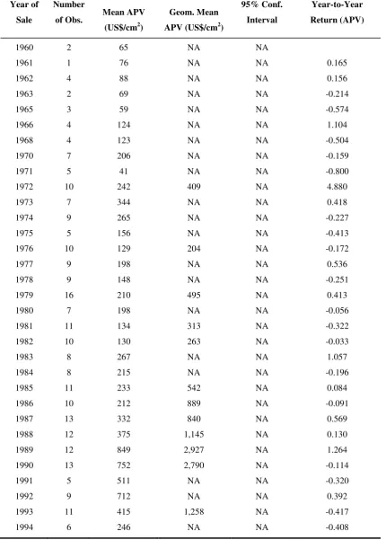
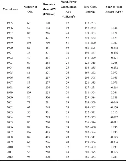
Returns for Different Artists or Group of Artists

Tables 8, 9 and 10 present the year-to-year returns for Renoir, Matisse and the

Impressionists (based on the information provided by data sets A, B and C respectively)

along with other key values. Notice the salient peak APV values (at year 1989 and then

around 2006) with their corresponding steep declines afterwards. They are consistent across

the three data sets and are in agreement with trends already detected in the broader art

market.

Return computations are straightforward. First, we compute for each year the

geometric mean of the APV values (GM-APV). This is simply the nth root of the product of

the APV-values associated with the n paintings sold during the year considered. Then, the

year-to-year returns are computed based on the GM-APV values for two consecutive years.

In short, the return between years i and i+1 is simply [GM-APVi+1/GM-APVi] – 1.

We have purposely carried out this calculation using the geometric mean and not the

conventional arithmetic mean. We think that using the geometric mean is more reasonable

since it is less sensitive to extreme values, something that becomes even more relevant when

the distributions depart significantly from normality (which is the case with the APV).

Leaving aside the ease of computation (undoubtedly an attractive feature) a valid

question needs to be answered: What does this return mean? The APV captures both, art

market trends and supply-demand dynamics for the artist or artists considered, as it is based

on actual sales. It does not intend to control the actual prices observed for any factor other

than the area of the painting. Hence, the APV-based returns can be interpreted as total (actual

or realized) returns for the artist or artists in question (inflation has been removed since prices

Table 8. Data set A: Pierre-Auguste Renoir, Key Statistics and Year-to-Year Returns

Year of Sale Number of Obs.

Geometric Mean APV (US$/cm2)

Stand. Error Geom. Mean APV

(US$/cm2)

95% Conf. Interval

Year-to-Year Return

(APV)

1985 32 267 57 154 - 379

1986 41 316 71 178 - 455 0.186

1987 83 436 94 252 - 620 0.377 1988 70 673 174 332 - 1015 0.546 1989 103 1043 258 537 - 1550 0.549 1990 93 919 217 493 - 1345 -0.119 1991 31 329 69 194 - 465 -0.642 1992 43 345 79 190 - 500 0.047 1993 56 338 90 162 - 514 -0.020 1994 45 309 51 208 - 410 -0.086 1995 75 279 60 162 - 396 -0.096 1996 69 244 53 140 - 348 -0.126 1997 75 351 90 174 - 528 0.438 1998 77 246 63 122 - 370 -0.299 1999 75 307 71 168 - 445 0.247 2000 75 340 79 187 - 494 0.110 2001 49 278 67 146 - 410 -0.183 2002 38 338 80 182 - 495 0.216 2003 44 328 64 202 - 454 -0.030 2004 63 309 68 177 - 442 -0.057 2005 79 368 55 261 - 475 0.190 2006 73 462 67 331 - 593 0.256 2007 94 516 96 328 - 704 0.117 2008 62 437 108 225 - 650 -0.153 2009 59 347 68 215 - 480 -0.205 2010 66 421 81 263 - 579 0.213 2011 66 382 81 222 - 542 -0.094 2012 84 384 88 211 - 557 0.006

*The 95% confidence interval was computed based on the standard error of the geometric mean for

Table 9. Data set B: Henri Matisse, Key Statistics and Year-to-Year Returns Year of Sale Number of Obs. Geometric Mean APV (US$/cm2)

Stand. Error Geom. Mean APV (US$/cm2)

95% Conf. Interval

Year-to-Year Return (APV)

1960 2 65 NA NA

1961 1 76 NA NA 0.165

1962 4 88 NA NA 0.156

1963 2 69 NA NA -0.214

1965 3 59 NA NA -0.574

1966 4 124 NA NA 1.104

1968 4 123 NA NA -0.504

1970 7 206 NA NA -0.159

1971 5 41 NA NA -0.800

1972 10 242 409 NA 4.880

1973 7 344 NA NA 0.418

1974 9 265 NA NA -0.227

1975 5 156 NA NA -0.413

1976 10 129 204 NA -0.172

1977 9 198 NA NA 0.536

1978 9 148 NA NA -0.251

1979 16 210 495 NA 0.413

1980 7 198 NA NA -0.056

1981 11 134 313 NA -0.322

1982 10 130 263 NA -0.033

1983 8 267 NA NA 1.057

1984 8 215 NA NA -0.196

1985 11 233 542 NA 0.084

1986 10 212 889 NA -0.091

1987 13 332 840 NA 0.569

1988 12 375 1,145 NA 0.130

1989 12 849 2,927 NA 1.264

1990 13 752 2,790 NA -0.114

1991 5 511 NA NA -0.320

1992 9 712 NA NA 0.392

1993 11 415 1,258 NA -0.417

Table 9. Data set B: Henri Matisse, Key Statistics and Year-to-Year Returns

(continued)

Year of Sale

Number of Obs.

Geometric Mean APV (US$/cm2)

Stand. Error Geom. Mean APV (US$/cm2)

95% Conf. Interval

Year-to-Year Return (APV)

1995 10 594 2,073 NA 1.420

1996 6 198 NA NA -0.668

1997 11 404 1,278 NA 1.044

1998 12 221 736 NA -0.452

1999 12 503 1,193 NA 1.274

2000 7 769 NA NA 0.528

2001 18 469 1,368 NA -0.390

2002 8 756 NA NA 0.613

2003 3 160 NA NA -0.788

2004 9 1,047 NA NA 5.526

2005 7 450 NA NA -0.570

2006 8 1,143 NA NA 1.540

2007 23 832 3,430 NA -0.272

2008 20 813 2,470 NA -0.023

2009 8 659 NA NA -0.189

2010 11 2,422 5,207 NA 2.673

2011 7 454 NA NA -0.813

2012 8 326 NA NA -0.281

*The 95% confidence interval was computed based on the standard error of the geometric mean for

each year. We required a sample size of at least 10 observations and that standard error of the

Table 10. Data Set C: Impressionists Group, Key Statistics and Year-to-Year Returns

Year of Sale Number of Obs.

Geometric Mean APV (US$/cm2)

Stand. Error Geom. Mean

APV (US$/cm2)

95% Conf. Interval

Year-to-Year Return (APV)

1985 60 170 17 137 - 203

1986 59 194 19 157 - 232 0.144

1987 85 286 24 239 - 333 0.471

1988 72 421 57 310 - 532 0.473

1989 149 719 51 618 - 820 0.707 1990 62 481 59 366 - 595 -0.332 1991 36 271 38 196 - 347 -0.436 1992 40 211 34 144 - 279 -0.221

1993 60 268 24 221 - 315 0.268

1994 61 206 25 156 - 255 -0.232

1995 81 221 26 169 - 272 0.072

1996 69 257 26 206 - 308 0.163

1997 87 277 29 221 - 333 0.079

1998 90 204 24 157 - 251 -0.264 1999 109 258 24 211 - 304 0.264

2000 80 306 40 229 - 384 0.189

2001 71 291 39 214 - 369 -0.049 2002 67 248 28 194 - 302 -0.150

2003 50 301 35 232 - 371 0.216

2004 75 293 31 232 - 355 -0.027 2005 86 290 28 236 - 344 -0.011

2006 89 376 38 302 - 450 0.296

2007 106 485 50 387 - 584 0.290 2008 89 415 49 319 - 511 -0.145 2009 62 276 40 198 - 354 -0.334

2010 73 329 37 257 - 402 0.193

2011 58 288 44 201 - 375 -0.125

2012 95 370 42 286 - 453 0.283

*The 95% confidence interval was computed based on the standard error of the geometric mean for

Table 11. Year-to-year returns based on the APV plus other relevant metrics

APV

Data Set A: Renoir

Data Set B : Matisse

Data Set C: Impressionists

Average APV Return (per Year) 5.14% 34.11% 6.61% Standard Deviation of Average Return 31.10% 118.26% 27.53% Cumulative Return* 43.94% 400.5% 117.47% Initial Year Geometric Mean APV (US$/cm2)** 267 65 170 Final Year Geometric Mean APV (US$/cm2)** 384 326 370

* Cumulative returns computed for 27 years for data sets A and C [1985-2012] and 52 years for data set B [1960-2012].

**Initial year-APV for data sets A and C is 1985 and for data set B is 1960. Final year-APV for all data sets is 2012

Table 11 summarizes the return results including both, average year-to-year returns,

and cumulative returns for the relevant time-periods. The easiness with which one can

compute these returns −contrasted, for example, with those estimated with HPMs (to be

discussed later)− is striking.

Repeat Sales Vis-à-Vis the Entire (All-Sales) Data Set

Many analysts have estimated returns using only data from repeat sales. As pointed

out before, a concern with this approach is that there could be a risk of selection bias. Table

12 shows the median APV values for each of the artists considered using: (i) all the

observations; and (ii) the repeat-sales subset. In two cases (Matisse and Renoir) the

differences in medians are significant at the 5% level. And, in four of the remaining six cases

the discrepancies are marginally significant (significant at the 10% level).

Finally, and somehow expectedly, the estimated returns (based, as before, on the

geometric mean of the APV-values) are quite different for the two groups. The fact that in

most cases the returns are higher when computed based on the repeat-sales set gives

credibility to the hypothesis that paintings are more likely to be sold if they have increased in

value.

These findings support the view that a selection bias cannot be ruled out when dealing

with repeat-sales data. Thus, return estimates based on repeat-sales regressions (despite the

claim that one has controlled for all the relevant factors) should be regarded with suspicion.

Table 12. Comparisons of APV medians and returns: all-sales versus repeat-sales for each

artist

All-sales Repeat-sales

Artist

Number of Sales

Median APV (US$/cm2)

Avg. Returns (per Year)

Number of Sales

Median APV (US$/cm2)

Avg. Returns (per Year)

Alfred Sisley 342 313 8.11% 118 327 19.84%

Camille Pissarro 586 338 8.01% 146 378 17.71%

Claude Monet 586 411 15.47% 176 476 27.54%

Henri Matisse 441 308 34.11% 160 249 24.00%

Odilon Redon 193 118 24.91% 36 91 35.06%

Paul Gauguin 167 465 42.93% 37 612 136.83%

Paul Signac 247 202 29.52% 90 180 23.79%

Pierre-Auguste Renoir 1,820 377 5.14% 426 425 10.11%

Validation of the APV Metric

A useful way to assess the validity of the new metric is to compare the results

obtained with the APV and those obtained with the commonly used hedonic models.

Returns

First, we estimate individual HPMs for each of the three cases (Renoir, Matisse, and

the Impressionists) using the entire corresponding data set. And second, we estimate the

returns based on the time-dummies of the corresponding hedonic model.

The HPMs employ the natural logarithm of the painting selling price as the dependent

variable. The independent variables (right-hand side of the regression equation) involve: (i)

linear and higher-order polynomial expressions based on the age of the artist at the time the

painting was executed; (ii) linear and higher-order polynomial expressions based on variables

associated with the geometry of the painting; and (iii) dummy (binary) variables associated

with the year the painting was sold, and, in the case of data set C, dummies to account for the

identity of the painter. The return between two consecutive years, say i+1 and i, is estimated

as exp(βi+1)/exp(βi) where the β’s denote the time-dummy coefficients of the hedonic

The corresponding adjusted R2’s (Renoir, Matisse, and Impressionists) are as follows:

0.75 (F= 137.47, p<.0001), 0.72 (F=18.78, p<.0001), and 0.72 (F= 99.87, p <.0001)

respectively. In addition, we used White’s (1980) test for heteroscedasticity and the null hypothesis of homoscedasticity in the least-squares residuals was not rejected in each of the

three samples (results can be provided upon request).

Table 13. Year-to-year returns: averages, standard deviations, and correlations (APV

and HPM)

Data Set A: Renoir

Data Set B : Matisse

Data Set C: Impressionists

Average APV Return (per Year) 5.14% 34.11% 6.61%

Standard Deviation of Average APV Return 31.10% 118.26% 27.53%

Average HPM Return (per Year) 6.61% 17.00% 9.62%

Standard Deviation of Average HPM Return 26.59% 65.72% 31.13%

Correlation APV Return- HPM Return 0.90 0.85 0.92

Table 13 shows the comparison between the average year-to-year return estimated

with (i) the APV metric; and (ii) the HPMs, as described before. In the case of Renoir and

the Impressionists both returns are close. This fact is also consistent with the high correlation

values reported, and the visual agreement displayed by the curves in Figures 5 and 7. In the

case of Matisse, both return curves (Figure 6) show the same tendencies and trends.

Figure 6. Year-to-year (APV and HPM) returns for Henri Matisse sales.

Figure 7. Year-to-year (APV and HPM) returns for Impressionists group sales.

However, the APV curve gives a better account of the peak values. This is in

agreement with the high correlation value reported (85% from Table 13) and the well-known

fact that time-dummies based-returns, since they take into consideration the entire dataset at

once (52 years in this case), tend to mitigate the effect of peaks and valleys, and thus, render

smoother curves. This explains, at least in part, the difference between the APV and the

HPM returns.

The high degree of consistency might seem surprising. However, the following two

observations can explain, appealing partly to intuition, the success of the APV: (1) regressing

the logarithm of the price on just the logarithm of the area of the painting, for the case of

Renoir, Matisse, and the Impressionists, we obtained adjusted R2’s values equal to 0.60, 0.35,

and 0.51 respectively. Recall that the R2’s values of the corresponding hedonic models were

0.75, 0.72, and 0.72 respectively. Hence, the APV metric −for all its roughness and

Monet, Matisse, Redon, Gauguin, Signac, and Renoir) we obtain the following (fairly high)

values: 0.41; 0.73; 0.67; 0.59; 0.66; 0.64; 0.76, and 0.77 respectively. These observations

provide some basis for making an argument that using the area of a painting as a

normalization factor is not that eccentric or bizarre; it has some sound foundation.

Life-Cycle Creativity Patterns

Hedonic models have also been used in the past to investigate the age at which an artist

produced its most valuable work. Typically, a HPM is fitted to the entire data available

(which normally cover several years) and then the natural logarithm of the average price

versus the artist’s age-at-the-time-the-painting-was-executed, based on such model, is plotted.

That is, the hedonic pricing equation is evaluated, for each age, using the average

characteristics corresponding to that age.

Figure 8. Life-Cycle Creativity Curve, Pierre-Auguste Renoir: Comparison between

(i) Log of APV profile and (ii) Log of Price (from HPM) profile

Figure 9. Life-Cycle Creativity Curve, Henri Matisse: Comparison between

Figure 10. Life-Cycle Creativity Curve, Claude Monet: Comparison between

(i) Log of APV profile and (ii) Log of Price (from HPM) profile

Figure 11. Life-Cycle Creativity Curve, Camille Pissarro: Comparison between (i) Log

of APV profile and (ii) Log of Price (from HPM) profile

Figures 8, 9, 10, and 11 compare the curves obtained: (i) using the above-mentioned

approach; and (ii) plotting the logarithm of the average APV versus age-at-execution. In this

case we used the average APV rather than the median, since the HPM-based curves are

normally done with the mean. The four artists considered were the only artists for whom we

had more than 400 sales observations: Renoir, Matisse, Monet, and Pissarro. All four graphs

show very consistent trends between the two curves. In essence, the HPM-curves do not

seem to offer anything more than the simpler APV-based curves show.

A more interesting point becomes obvious when we compare these life-cycle curves

with those displayed before in Figs. 1, 2, 3, and 4 which were obtained using the median

extent, this is to be expected, as the log-function tends to mitigate the effect of peaks and

valleys. Furthermore, this phenomenon calls into question the benefits of building these

curves using the log-function (regardless of the underlying variable) instead of using the real

thing, that is, the actual variable −for example the APV (with no log applied).

To sum up, the APV-based calculations, in all cases considered, yielded very similar

results to those obtained with the hedonic models. This provides good evidence that the APV

metric, despite its simplicity, offers results consistent with conventionally accepted methods.

Suggestions for Future Applications

APV-based Derivatives and Index Contracts

The market for paintings lacks a widely accepted index or indices that could be used to

design derivatives contracts for hedging and/or speculative purposes. We reckon that the

reason is that the most popular indices (Mei-Moses index, artnet.com family of indices, AMR

indices, etc.) while effective for the purpose they were designed −namely, tracking broad

market trends− are unsuitable for financial contracts. The reason is that they involve certain

elements (proprietary databases, discretionary rules in terms of which sales should be

included, ad hoc combinations of repeat sales techniques coupled with some undesirable

features of HPMs) that make them opaque and −at least in theory− vulnerable to

manipulation. In contrast, indices such as the S&P 500 or the Barclays Capital bond indices

family −which are based on well-defined and transparent rules− are easy to reproduce and difficult to game. Not surprisingly, derivatives contracts based on these indices have enjoyed

wide market acceptance.

We think that the APV metric provides a natural tool to create well-defined indices that

could be the foundation for a derivatives art market. If one wishes to design an index to

represent a specific market segment −for example, the Impressionists− the main point is to agree on the artists that should be part of the index. Once this issue is settled −a rule that

must stay unaltered over time− what remains to agree upon is simply a mechanistic recipe to

calculate the value of the index. For instance, it could be the average APV value of all the

paintings sold in public auctions in the last twelve months as long as their values exceeded

US$ 50,000.

A contract built around an index of this type could be used to gain exposure to this

that sense, these types of contracts could help to expand the investor base, and contribute to

improve market liquidity. The operational details are similar, for instance, to those

encountered in the agricultural derivatives market or commodities markets. This topic is

presently under investigation by the authors.

Testing the CAPM Validity in the Art Market

Several authors have investigated the validity of the CAPM model within the context

of the art market. Although the results have been mixed we also think they have been

irrelevant. The reason is that most authors —erroneously in our view— have placed on the

left-hand side of the CAPM equation estimates of returns obtained, in general, via the

time-dummy coefficients of a suitable hedonic model. We reckon that the correct approach is to

place on the left-hand side of the CAPM equation estimates of total returns—not returns

based on the time-dummies—which, at best, seem to capture (although this topic is still

subject to debate) market returns. Total returns, of course, can be easily estimated with the

APV metric.

This suggestion might sound strange until one realizes that, for instance, if we were to

apply the CAPM model to, say, IBM’s stock ,we would place on the left-hand side of the

equation the return based on the price of IBM stock over some time period: in short, the total

return. We would never place on the left-hand side the IBM stock return computed after

controlling for whatever market factors might influence it (composition of revenue, number

of employees, technology changes, etc.)

Moreover, most researchers never account for the fact that returns estimated via the

time-dummies are just estimates, and therefore, subject to error. Obviously, this error

translates itself into an additional error when estimating the CAPM's betas. Add to this the

possibility of spurious return estimates as a result of the violation of the monotonicity

condition, and inevitably one needs to wonder about the meaning or validity of such

CAPM-related findings.

In summary, it is quite odd that the validity of the CAPM within the art market

context has been carried out using returns that: (i) do not capture supply-demand changes

from period-to-period; and (ii) could be contaminated by spurious effects due to the violation

Conclusions

We have introduced an easy-to-compute financial metric suitable for two-dimensional

art objects that is both intuitive and transparent. It has several appealing features: it is

difficult to game since not much discretion comes into its evaluation (unlike hedonic models

that are data intensive and often exhibit lack of stability); it can be applied to artists for whom

there are few observations, albeit with all the caveats appropriate for small data sets; it

facilitates comparisons between artists, between different types of paintings by the same

artist, or, paintings done by the same artist at different life-periods; it is also appropriate to

explore artists’ consistency, by looking at its standard deviation or coefficient of variation; and, finally, it can be employed to construct well-defined total-return indices to create

financial derivatives.

However, it must be emphasized that the main goal of this new metric is to offer an

investor a useful yardstick that captures, after normalizing by the area, a representative price.

It is not the aim of the APV to control prices for other characteristics or to build a market

index based on a time-independent ideal painting. For these reasons the APV metric is

ideally suited to compute actual returns.

In terms of estimating returns, the APV metric offers three attractive features: (i)

unlike repeat-sales regression models, it uses all the available data; (ii) unlike HPMs, whose

effectiveness can depend substantially on the variables chosen and the analyst’s skill to select

them, the APV gives a unique value: the actual total return; and (iii) APV-based returns can

always be computed regardless of the number of observations. On the other hand,

HPM-based returns can be computed only in the limited number of cases where one has enough

data, with the caveat that the accuracy of such returns estimates is weakened by the

explicatory power of the relevant model since the R2 is never 1.

Although the topic of this paper has been to introduce a new tool to the analyst’s

toolkit, rather than questioning the virtues of the HPMs in the context of the art market, one

thing is obvious: hedonic models, considering how data-intensive they are plus the additional

limitations already mentioned, do not seem to offer a lot more insight than the simple APV

metric −at least for the examples discussed in this study. Moreover, the high correlation

observed between returns computed using the APV and those based on HPMs reinforces this

In summary, we hope investors, financial analysts, and future researchers will be able

to explore −and exploit− the merits of the APV metric. Our goal has been simply to

introduce the tool, showcase a few applications, and perform some validation tests.

Finally, the main advantage of the APV is that it is a financial metric and not a

modeling technique; therefore, it is what it is, and it can always be computed. In short, it can

be useful or useless, but never wrong.

References

Agnello, R. J. and Pierce, R. K. 1996. “Financial returns, price determinants, and genre effects in American art investment”. Journal of Cultural Economics, vol. 20, no. 4 (December):359–383.

Anderson, R. C. 1974. “Paintings as an investment”. Economic Inquiry, vol. 12, no. 1 (January):13–26.

artnet Analytics. 2012. “artnet Indices White Paper”.

www.artnet.com/analytics/reports/white-paper

Ashenfelter, O. and Graddy, K. 2003. “Auctions and the price of art”. Journal of Economic Literature, vol. 41, no. 3 (September):763–786.

Baumol, W. J. 1986. “Unnatural value: Or art investment as a floating crap game”. American Economic Review, vol. 76, no. 2 (May):10–14.

Bonnet, D. G. and Price, R. M. 2002. “Statistical inference for a linear function of medians:

Confidence intervals, hypothesis testing, and sample size requirements”.

Psychological Methods, 7(3), 370–383.

Brachinger, H. W. 2003. “Statistical Theory of Hedonic Price Indices”. DQE Working Papers 1, Department of Quantitative Economics, University of Freiburg/Fribourg

Switzerland.

Campos, N. F. and Barbosa, R. L. 2009. “Paintings and numbers: an econometric

investigation of sales rates, prices, and returns in Latin American art auctions”.

Oxford Economic Papers, vol. 61, no. 1 (January):28–51.

Chanel, O., Gerard-Varet, L. A., and Ginsburgh, V. 1994. “Prices and returns on paintings:

An exercise on how to price the priceless”. The Geneva Risk and Insurance Review, vol. 19, no. 1 (June):7–21.

Chanel, O., Gerard-Varet, L. A., and Ginsburgh, V. 1996. “The relevance of hedonic price

Coate, B. and Fry, T. L. R. 2012. “Better off Dead? Prices realised for Australian Paintings

Sold at Auction”. ACEI Working Paper Series, AWP-2-2012. Available online: http://www.culturaleconomics.org/workingpapers.html.

Collins, A., Scorcu, A. E., and Zanola, R. 2007. “Sample Selection Bias and Time

Instability of Hedonic Art Price Indices”. Working papers DSE No. 610.

de Haan, J. and Diewert, E. 2011. “Hedonic Regression Methods”. In: de Haan, J. and

Diewert, E., eds. Handbook on Residential Property Prices Indices. (November)

http://epp.eurostat.ec.europa.eu/portal/page/portal/hicp/methodology/hps/rppi_handbo

ok

de la Barre, M., Docclo, S., and Ginsburgh, V. 1994. “Returns of impressionist, modern and

contemporary European paintings 1962–1991”. Annales d’Economie et de

Statistique, vol. 35 (July-September):143–181.

Edwards, S. 2004. “The Economics of Latin American Art: Creativity Patterns and Rates of Return”. Economía, vol. 4, no. 2, (Spring): 1-35.

Ekelund, R., Ressler, R., and Watson, J. 2000. “The ‘‘death-effect’’ in art prices: A demand

-side exploration”. Journal of Cultural Economics, 24, no. 4 (November):283–300.

Fisher, I. 1922. The Making of Index Numbers; a Study of their Varieties, Tests, and

Reliability. Boston: Houghton-Mifflin.

Galbraith, J. W. and Hodgson, D. 2012. “Dimension reduction and model averaging for

estimation of artists' age-valuation profiles”. European Economic Review, vol. 56,

no. 3 (April):422–435.

Galenson, D. W. 1999. “The Lives of the Painters of Modern Life: The Careers of Artists in

France from Impressionism to Cubism”. NBER Working Paper 6888. Galenson, D. W. 2000. “The careers of modern artists. Evidence from auctions of

contemporary art”. Journal of Cultural Economics, vol.24, no. 2 (May):87–112. Galenson, D. W. 2001. Painting Outside the Lines: Patterns of Creativity in Modern Art.

Harvard University Press

Galenson, D. W. and Weinberg B. A. 2000. “Age and the Quality of Work: The Case of

Modern American Painters”. Journal of Political Economy, vol. 108, no. 4 (August):761–777.

Ginsburgh, V., Mei, J., and Moses M. 2006. “The computation of price indices”. In

Handbook of the Economics of Art and Culture, edited byGinsburgh, V.A. and

Ginsburgh, V. and Weyers, S. 2006. “Creativity and life cycles of artists”. Journal of

Cultural Economics, vol. 30, no. 2 (September):91–107.

Goetzmann, W.N. 1993. “Accounting for taste: art and financial markets over three centuries”. American Economic Review, vol. 83, no. 5 (December):1370–1376.

Higgs, H. and Forster, J. 2013. “The auction market for artworks and their physical

dimensions: Australia—1986 to 2009”. Journal of Cultural Economics, January 11:

doi 10.1007/s10824-012-9197-z.

Higgs, H. and Worthington, A. C. 2005. “Financial returns and price determinants in the

Australian art market, 1973–2003”. The Economic Record, vol. 81, no. 253

(June):113–123.

Mei, J. and Moses, M. 2002. “Art as an investment and the underperformance of

masterpieces”. American Economic Review, vol. 92, no. 5 (December):656–1668.

Melser, D. 2005. “The Hedonic Regression Time-Dummy Method and the Monotonicity

Condition.” Journal of Business & Economics Statistics, 23, 485–492.

Pesando, J. E. 1993. “Arts as an investment: The market for modern prints”. American Economic Review, vol. 83, no. 5 (December):1075–1089.

Price, R. M. and Bonett, D. G. 2001. “Estimating the variance of the median”. Journal of Statistical Computation and Simulation, vol. 68, no. 3:295–305.

Renneboog, L. and Spaenjers, C. 2013. “Buying beauty: On prices and returns in the art market”. Management Science, vol. 59, no. 1 (January):36–53

Renneboog, L. and Spaenjers, C. 2011. “The iconic boom in modern Russian art”. Journal of Alternative Investments, vol. 13, no. 3 (Winter):67–80.

Renneboog, L. and Van Houtte, T. 2002. “The monetary appreciation of paintings: From realism to Magritte”. Cambridge Journal of Economics, 26(3), 331–357.

Scorcu, A. E. and Zanola, R. 2011. “The “Right” Price for Art Collectibles: A Quantile

Hedonic Regression Investigation of Picasso Paintings”. The Journal of Alternative Investments, vol. 14, no. 2 (Fall):89–99.

Sproule, R. and Valsan C. 2006. “Hedonic models and pre-auction estimates: Abstract art

revisited”. Economics Bulletin, vol. 26, no. 5 (November):1–10.

White, H. 1980. “A heteroscedasticity-consistent covariance matrix and a direct test for

Wilcox, R. R. 2005. “Comparing medians: An overview plus new results on dealing with

heavy-tailed distributions”. The Journal of Experimental Education, vol. 73, no. 3

(August): 249-263.

Worthington, A. C. and Higgs, H. 2004. “Art as an investment: Risk, return and portfolio