The Rational Solutions and the Interactions of the N Soliton Solutions for Boiti Leon Manna Pempinelli Like Equation

http://www.scirp.org/journal/jamp

ISSN Online: 2327-4379 ISSN Print: 2327-4352

The Rational Solutions and the Interactions of

the N-Soliton Solutions for

Boiti-Leon-Manna-Pempinelli-Like Equation

Xiuxiu Liu, Huanhe Dong, Yong Zhang, Xin Chen

Department of Mathematics and Systems Science, Shandong University of Science and Technology, Qingdao, China

Abstract

These rational solutions which can be described a kind of algebraic solitary waves which have great potential in applied value in atmosphere and ocean. It has attracted more and more attention recently. In this paper, the generalized bilinear method instead of the Hirota bilinear method is used to obtain the ra-tional solutions to the (2 + 1)-dimensional Boiti-Leon-Manna-Pempinelli-like equation (hereinafter referred to as BLMP equation). Meanwhile, the (2 + 1)-dimensional BLMP-like equation is derived on the basis of the generalized bilinear operators D3,x,D3,y and D3,t. And the rational solutions to the (2 +

1)-dimensional BLMP-like equation are obtained successively. Finally, with the help of the N-soliton solutions of the (2 + 1)-dimensional BLMP equation, the interactions of the N-soliton solutions can be derived. The results show that the two soliton still maintained the original waveform after happened collision.

Keywords

Rational Solution, Generalized Bilinear Method, BLMP-Like Equation, N-Soliton Solution

1. Introduction

In recent years, with the emergence of high-powered computer and the develop-ment of mathematical research, various nonlinear problems increasingly cause at-tentions of scientists. Especially some key problems in engineering, science and modern physics are ultimately dependent on the specific solution of the nonlinear equations. So the solution of the nonlinear equations [1] [2] [3] [4] [5] occupies very important position no matter on theory research or practical application. But the diverse nonlinear equations of mathematical physics was descried with Hirota bilinear equations [6] [7] [8] and generalized bilinear equations [9] [11] [12] [13],

How to cite this paper: Liu, X.X., Dong, H.H., Zhang, Y. and Chen, X. (2017) The Rational Solutions and the Interactions of the N-Soliton Solutions for Boiti-Leon- Manna-Pempinelli-Like Equation. Journal of Applied Mathematics and Physics, 5, 700-714.

https://doi.org/10.4236/jamp.2017.53059

Received: February 16, 2017 Accepted: March 28, 2017 Published: March 31, 2017

Copyright © 2017 by authors and Scientific Research Publishing Inc. This work is licensed under the Creative Commons Attribution International License (CC BY 4.0).

http://creativecommons.org/licenses/by/4.0/

such as the KdV equations [10] [11] [14] [15], the BLMP equations [16] [17] [18], the NLS equation, the Boussinesq equation [19], the KP equations [9] [20] [21] and so on. There has been a growing attention on rational solutions [2] [3] [9] [10] [11] [22] to nonlinear differential equations in recent years. One kind of particular rational solutions are rogue wave solutions [24] [25] [26], which describe signifi-cant nonlinear wave phenomena in oceanography. So the rational solutions of the nonlinear equations become crucial in atmosphere and ocean.

As we know some rational solutions to integrable equations have been consi-dered systematically on the basis of the Wronskian formulation, the Casoratian formulation and the Pfaffian formulation [9]. Rational solutions to the nonlinear differential equation are also considered by different approaches, such as the G G′ expansion methods [9] [10] [27] and the tanh-coth function method [28]. Moreover, the Hirota method is also used to construct rational solutions to the nonlinear differential equations. And it is very necessary and interesting for us to study rational solutions and generate the generalized bilinear form to non-linear differential equations.

In this paper, the rational solutions to the (2 + 1)-dimensional BLMP equa-tion can be derived by the Hirota bilinear method. And the (2 + 1)-dimensional BLMP-like nonlinear differential equation on the basic of existing BLMP bilinear differential equation can be derived via applying three generalized bilinear oper-ators D3,x,D3,y and D3,t. Later, the rational solutions to the BLMP-like equation

are obtained by Maple computation. Finally, the N-soliton solutions [4] [8] [29] to the (2 + 1)-dimensional BLMP equation are given under the Hirota method.

2. Hirota Bilinear D-Operators and the Rational Solutions to

the (2 + 1)-Dimensional BLMP Equation

2.1. Hirota Bilinear D-Operators

The D-operators are defined in Refs. [6] [7] [8] as following:

(

) (

) ( ) (

)

,

, , ,

m n

m n

x t x x t t

x x t t

D D F G _{′ ′} F x t G x t

′ ′ = =

′ ′

⋅ = ∂ − ∂ ∂ − ∂ (1)

where m n, are all non-negative integer.

Assume m=1,n=0, Equation (1) can be reduced to

.

x x x

D F G⋅ =F G−FG (2) Assume m=1, 1,n= Equation (1) can be reduced to

.

x t xt t x x t xt

D D F G⋅ =F G−F G −F G +FG (3) 2.2. The Rational Solutions to the (2 + 1)-Dimensional BLMP

Equation

Consider a (2 + 1)-dimensional BLMP equation

3 3 0,

yt xxxy xx y x xy

u +u − u u − u u = (4) according to the formula Equation (1), the bilinear form as follows

(

3

)

0,

y t x y

D D +D D F F⋅ = (6) under the transformation u= −2 ln

(

F

)

_x.

Apply the direct Maple symbolic computation 3 2 2

0 0 0

,

i k t ijk i j k

F c x y t

= = =

=

∑∑∑

(7)

to obtain the polynomial solutions to Equation (5). where the cijk are constants.

The twelve classes of polynomial solutions to Equation (4) are obtained, as follows.

The first class of rational solutions to Equation (4):

1

m u

n

−

= (8) there

(

2 2 2 2 2 2

)

3,2,1 2,2,1 3,1,1 1,2,1 2,1,1 3,0,1 1,1,1 2,0,1 1,0,1

2 3 2 2 3 2 2 3 2 2

3,2,1 2,2,1 3,1,1 1,2,1 2,1,1 3,0,1 0,2,1 1,1,1 2,0,1 0,1,1 1,0,1 0,0

2 3 2 3 2 3 2 ,

m t x c t xc tx c t c txc x c tc xc c

n t x c t x c tx c t xc tx c x c t c txc x c tc xc c

= + + + + + + + +

= + + + + + + + + + + + ,1.

The second class:

2

m u

n

−

= (9) there

(

2 2 2 2 2 2

2,0,1 3,0,2 2,0,2 3,0,1 3,0,2 2,0,1 3,0,1 3,0,2

2 2 2 2 2

2,0,2 3,0,1 2,0,1 2,0,2 3,0,2 2,0,2 3,0,1

2 2 2

2,0,1 3,0,0 3,0,2 2,0,2 3,0,0 3,0,1 2,0,1 3,0,2

2,0,

6 3 3 3

3 2 2

3 3 2

2

m x y c c x y c c c x yc c c

x yc c xy c c c xy c c

x c c c x c c c xyc c

xyc

= − +

− + −

+ − +

− 2 2

1 2,0,2 3,0,1 1,0,2 2,0,1 3,0,2 1,0,2 2,0,2 3,0,1

2,0,0 2,0,1 3,0,2 2,0,0 2,0,2 3,0,1 1,0,1 2,0,1 3,0,2

1,0,1 2,0,2 3,0,1 1,0,1 2,0,0 3,0,2 1,0,1 2,0,2 3,0,0

1,0,2 2,0,0 3,0,1 1

2 2

c c y c c c y c c c

xc c c xc c c yc c c

yc c c c c c c c c

c c c c

+ −

+ − +

− + −

− + _{,0,2 2,0,1 3,0,0}

)

_{3,0,2 3,1,2}

3 2 3 3 2 2 3 2

2,0,1 3,0,2 3,1,2 2,0,2 3,0,1 3,0,2 3,1,2 2,0,1 3,0,1 3,0,2 3,1,2

3 2 2 2 2

2,0,2 3,0,1 3,0,2 3,1,2 2,0,1 2,0,2 3,0,2 3,1,2 2 2 2

2,0,2 3,0,1 3

,

3 3 3

3 3

3

c c c c

n x y c c c x y c c c c x yc c c c x yc c c c x y c c c c

x y c c c

= − +

− +

− 2 3

,0,2 3,1,2 2,0,1 3,0,2 3,1,2

2 2 3 2

2,0,2 3,0,1 3,0,2 3,1,2 2,0,1 3,0,0 3,0,2 3,1,2

3 2 2 2

2,0,2 3,0,0 3,0,1 3,0,2 3,1,2 2,0,1 3,0,2 3,1,2

2 2

2,0,1 2,0,2 3,0,1 3,0,2 3,1,2 1, 36

36 3

3 3

3 3

c ty c c c

ty c c c c x c c c c x c c c c c x yc c c x yc c c c c xy c

+

− +

− +

− + 2

0,2 2,0,1 3,0,2 3,1,2

2 2

1,0,2 2,0,2 3,0,1 3,0,2 3,1,2 2,0,1 3,0,1 3,0,2 3,1,2

2 2 2

2,0,2 3,0,1 3,0,2 3,1,2 2,0,0 2,0,1 3,0,2 3,1,2 2

2,0,0 2,0,2 3,0,1 3,0,2 3,1,2 1,0,1 2,0,1

3 36

36 3

3 3

c c c xy c c c c c tyc c c c

tyc c c c x c c c c x c c c c c xyc c c

− +

− +

− + 2

3,0,2 3,1,2

2 3

1,0,1 2,0,2 3,0,1 3,0,2 3,1,2 0,1,2 2,0,1 3,0,2

2 2 2 4 2 3

0,1,2 2,0,2 3,0,1 3,0,2 2,0,1 3,0,2 2,0,2 3,0,1 3,0,2 2

2,0,1 3,0,0 3,0,2 3,1,2 2,0,2 3,0,0 3,0,1 3,0,2

3 3

3 36 36

36 36

c xyc c c c c y c c c

y c c c c y c c y c c c

tc c c c tc c c c

− +

− − +

+ − 2

3,1,2 1,0,1 2,0,0 3,0,2

1,0,1 2,0,2 3,0,0 3,0,2 3,1,2 1,0,2 2,0,0 3,0,1 3,0,2 3,1,2

2 2

1,0,2 2,0,1 3,0,0 3,0,2 3,1,2 0,1,2 2,0,1 3,0,1 3,0,2 0,1,2 2,0,2 3,0,1 3,0,2

1,0,1 2,0,1

3

3 3

3 3 3

c xc c c

xc c c c c xc c c c c

xc c c c c yc c c c yc c c c

yc c

+

− −

+ + −

+ 2 2

2,0,2 3,0,2 3,1,2 1,0,1 2,0,2 3,0,1 3,1,2 1,0,2 2,0,1 3,0,2 3,1,2

3 2 2

1,0,2 2,0,1 2,0,2 3,0,1 3,1,2 2,0,1 3,0,1 3,0,2 2,0,2 3,0,1 3,0,2 2

0,1,2 2,0,1 3,0,0 3,0,2 0,1,2 2,0,2 3,0,0

36 36

3 3

c c c yc c c c yc c c c

yc c c c c yc c c yc c c

c c c c c c c

− −

+ − +

+ − _{3,0,1 3,0,2 1,0,1 2,0,0 2,0,2 3,0,2 3,1,2}

2

1,0,1 2,0,2 3,0,0 3,1,2 1,0,2 2,0,0 2,0,1 3,0,2 3,1,2 1,0,2 2,0,1 2,0,2 3,0,0 3,1,2

3 2

2,0,1 3,0,0 3,0,2 2,0,2 3,0,0 3,0,1 3,0,2

36 36 .

c c c c c c c

c c c c c c c c c c c c c c

c c c c c c c

+

− − +

The third class: 3 m u n −

= (10) there

(

2 2 2 2 2 2

2,1,2 3,0,2 3,0,2 2,1,2 3,0,1 1,1,2 3,0,2 3,0,1 3,0,2

2 2

2,0,2 3,0,2 2,1,2 3,0,0 1,1,2 3,0,1 3,0,0 3,0,2 2,0,2 3,0,1 2

1,0,2 3,0,2 1,1,2 3,0,0 2,

2 2 3 2 3

2 2 3 2

2

m txy c c x y c txyc c ty c c x yc c

xy c c txc c tyc c x c c xyc c

y c c tc c xc

= + + + +

+ + + + +

+ + +

)

3

0,2 3,0,0 1,0,1 3,0,2 1,0,0 3,0,2 2,1,2 3,0,2

2 2 4 2 3 2 3 3 2 4 2 3 2

2,1,2 3,0,2 2,1,2 3,0,2 2,1,2 3,0,1 3,0,2 1,1,2 2,1,2 3,0,2

3 3 2 2 2 3 2 2 4

2,1,2 3,0,1 3,0,2 2,0,2 2,1,2 3,0,2 2,1,2

,

c yc c c c c c

n tx y c c x y c c tx yc c c txy c c c

x yc c c x y c c c tx c

+ +

= + + +

+ + + 3

3,0,0 3,0,2 1,1,2 2,1,2 3,0,1 3,0,2

2 4 2 2 2 2 2 3 2 3 3

1,0,2 2,1,2 3,0,2 1,1,2 2,1,2 3,0,2 1,1,2 2,0,2 2,1,2 3,0,2 2,1,2 3,0,2

3 3 2 2 3 2

2,1,2 3,0,0 3,0,2 2,0,2 2,1,2 3,0,1 3,0,2 1,0,

12

c c txyc c c c

ty c c c ty c c c ty c c c c ty c c

x c c c x yc c c c x c

+

+ + − +

+ + + 3 2 3

2 2,1,2 3,0,2 1,1,2 2,1,2 3,0,0 3,0,2

4 2 2 3 3 2

1,0,1 2,1,2 3,0,2 1,1,2 2,1,2 3,0,1 3,0,2 1,1,2 2,0,2 2,1,2 3,0,1 2,1,2 3,0,1 3,0,2

2 3 3 2

2,0,2 2,1,2 3,0,0 3,0,2 1,0,1 2,1,2 3,0,2

12

c c txc c c c

tyc c c tyc c c c tyc c c c tyc c c

x c c c c xyc c c

+

+ + − +

+ + 2 2 2

1,0,2 1,1,2 2,1,2 3,0,2

2 3 2 3 3 2 2 2 2 2 2

1,0,2 2,0,2 2,1,2 3,0,2 1,1,2 3,0,2 1,1, 2,0,2 2,1,2 3,0,2 1,1,2 2,0,2 2,1,2 3,0,2

2 4 2 2 3 4

1,1,2 2,1,2 3,0,2 2,0,2 2,1,2 3,0,2 1,0,0 2,1,2 3

2

18 12

y c c c c

y c c c c y c c y c c c c y c c c c

y c c c y c c c tc c c

−

+ − + −

− + + 2 2

,0,2 1,1,2 2,1,2 3,0,0 3,0,2

3 3 2 3 2 2 2

1,1,2 2,0,2 2,1,2 3,0,0 2,1,2 3,0,0 3,0,2 1,0,0 2,1,2 3,0,2 1,0,1 1,1,2 2,1,2 3,0,2

3 3 2 2

1,0,1 2,0,2 2,1,2 3,0,2 1,1,2 3,0,1 3,0,2 1,1,2 2,0,2

12

2

tc c c c

tc c c c tc c c xc c c yc c c c

yc c c c yc c c yc c

+

− + + −

+ − + 2,1,2 3,0,1 3,0,2

2 2 3 2 2

1,1,2 2,0,2 2,1,2 3,0,1 1,1,2 2,1,2 3,0,1 3,0,2 2,0,2 2,1,2 3,0,1 3,0,2

2 2 3 3 2 2

1,0,0 1,1,2 2,1,2 3,0,2 1,0,0 2,0,2 2,1,2 3,0,2 1,1,2 3,0,0 3,0,2 1,1,2 2,0,2 2,1

18 12

2

c c c

yc c c c yc c c c yc c c c

c c c c c c c c c c c c c c

− − +

− + − + _{,2 3,0,0 3,0,2}

2 2 3 2 2

1,1,2 2,0,2 2,1,2 3,0,0 1,1,2 2,1,2 3,0,0 3,0,2 2,0,2 2,1,2 3,0,0 3,0,2

18 12 .

c c

c c c c c c c c c c c c

− − +

The fourth class:

4

m u

n

−

= (11) there

(

2 2

)

3,0,1 2,0,1 1,0,2 1,0,1 1,0,0 3,0,1

3 2 2 2 2

3,0,1 2,0,1 3,0,1 1,0,2 3,0,1 3,0,1 1,0,1 3,0,1 2

1,0,2 2,0,1 1,0,0 3,0,1 0,0,1 3,0,1 1,0,0 2,0,1

6 3 2 ,

3 3 3 36 3

3 3 .

m x yc xyc y c yc c c

n x yc x yc c xy c c tyc xyc c

y c c xc c yc c c c

= + + + +

= + + + +

+ + + +

The fifth class:

5

m u

n

−

= (12) there

(

2 2

)

2,0,2 3,0,1 2,0,2 2,0,1 2,0,2 1,0,2 2,0,2 0,0,2 3,0,1 1,0,2 2,0,1

3 2 2 2

2,0,2 3,0,1 2,0,2 2,0,1 2,0,2 1,0,2 2,0,2 2,0,2 3,0,1

0,0,2 3,0,1 1,0,2 2,0,1 0,0,2 2,

2 3 2 2 3 ,

12 3

m x c c xyc xc c yc c c c c c

n x c c x yc x c c xyc c tc c

xc c xc c yc c

= + + + − +

= + + + +

− + + _0,2+c_{0,0,1 2,0,2}c .

The sixth class:

6

m u

n

−

there

(

)

2

(

2

2,0,1 3,1,1 2,1,1 3,0,1 1,0,2 1,0,2 2,0,1 3,0,1 3,1,1 1,0,2 2,1,1 3,0,1

2 3 2 2

1,0,2 3,0,1 0,0,2 2,0,1 3,0,1 3,1,1 0,0,2 2,1,1 3,0,1 1,0,2 2,0,1 3,1,1

1,0,2 2,0,1 2,1,1 3,0,1

2 2 2

3

2

m c c c c c txc c c c txc c c

x c c tc c c c tc c c tc c c

tc c c c

= − −

− − + +

− − 2 2 2 2

)

1,0,2 2,0,1 3,0,1 1,0,2 3,0,1 1,0,1 1,0,2 3,0,1

2 3 2 2 2 3 2 2 3 2 3

1,0,2 2,0,1 3,0,1 3,1,1 1,0,2 2,0,1 2,1,1 3,0,1 3,1,1 1,0,2 2,1,1 3,0,1

3 3 3 3 3

1,0,2 2,0,1 3,0,1 3,1,1 1,0,2 2,1,1 3,

, 2

xc c c yc c c c c

n tx c c c c tx c c c c c tx c c c

x c c c c x c c c

− −

= − +

− + 4 2 2 2

0,1 0,0,2 1,0,2 2,0,1 3,0,1 3,1,1

2 2 2 2 3 3 3 2

0,0,2 1,0,2 2,0,1 2,1,1 3,0,1 3,1,1 0,0,2 1,0,2 2,1,1 3,0,1 1,0,2 2,0,1 3,1,1

3 2 3 2

1,0,2 2,0,1 2,1,1 3,0,1 3,1,1 1,0,2 2,0,1 2,1,1 3,

2 2

txc c c c c

txc c c c c c txc c c c txc c c

txc c c c c txc c c c

−

+ − +

− + 2 4 2 2

0,1 1,0,2 2,0,1 3,1,1

4 4 2 2 2 3 2 2

1,0,2 2,0,1 2,1,1 3,0,1 3,1,1 1,0,2 2,1,1 3,0,1 1,0,2 2,0,1 3,0,1 3,1,1

2 3 3 4 2 4 3

1,0,2 2,0,1 2,1,1 3,0,1 1,0,2 2,0,1 3,0,1 3,1,1 1,0,2 2,1,1 3,0,1

2

tyc c c

tyc c c c c tyc c c x c c c c

x c c c c xyc c c c xyc c c

+

− + −

+ − +

2 2 2 2 2 2 2 3

0,0,2 1,0,2 2,0,1 3,0,1 3,1,1 0,0,2 1,0,2 2,0,1 2,1,1 3,0,1 3,1,1 0,0,2 1,0,2 2,1,1 3,0,1

2 3 2 2 2 2

0,0,2 1,0,2 2,0,1 3,1,1 0,0,2 1,0,2 2,0,1 2,1,1 3,0,1 3,1,1 0,0,2 1,0,2 2,0,1 2

2 2

tc c c c c tc c c c c c tc c c c

tc c c c tc c c c c c tc c c c

+ − +

− + − 2 2

,1,1 3,0,1

3 2 2 3 3 2 2

1,0,1 1,0,2 2,0,1 3,1,1 1,0,1 1,0,2 2,0,1 2,1,1 3,0,1 3,1,1 1,0,1 1,0,2 2,1,1 3,0,1

3 3 3 4 3 2

1,0,2 2,0,1 3,0,1 3,1,1 1,0,2 2,1,1 3,0,1 1,0,1 1,0,2 2,0,1 3,0,1 3,1,1

2

12 12

c

tc c c c tc c c c c c tc c c c

tc c c c tc c c xc c c c c

+ − +

− + −

3 3 3 2 3 3

1,0,1 1,0,2 2,1,1 3,0,1 0,0,2 1,0,2 2,0,1 3,0,1 3,1,1 0,0,2 1,0,2 2,1,1 3,0,1

3 3 3 4 2 2 2

0,0,2 2,0,1 3,0,1 3,1,1 0,0,2 2,1,1 3,0,1 0,0,2 1,0,2 2,0,1 3,0,1 3,1,1 2

0,0,2 1,0,2 2,0,1 2,1,

xc c c c yc c c c c yc c c c

c c c c c c c c c c c c

c c c c

+ − +

− + +

− 3 2 2 2 3

1 3,0,1 0,0,2 1,0,1 1,0,2 2,0,1 3,0,1 3,1,1 0,0,2 1,0,1 1,0,2 2,1,1 3,0,1

2 5 3 4

0,0,2 1,0,2 3,0,1 1,0,2 2,0,1 3,0,1

18 6 .

c c c c c c c c c c c c

c c c c c c

− +

+ −

The seventh class:

7

m u

n

= (14) there

(

2

)

3,0,1 2,0,1 1,0,1

3 2 2

3,0,1 2,0,1 3,0,1 1,0,1 0,0,2 0,0,1 0,0,0

2 3 2 ,

6 .

m x c xc c y

n x yc x yc tyc xyc y c yc c

= + +

= − − + − − − −

The eighth class:

8

m u

n

−

= (15) there

(

2 2 2

)

2,2,2 3,1,2 1,2,2 2,1,2 1,1,2 1,0,2

2 2 3 2 2

2,2,2 3,1,2 1,2,2 2,1,2

2

0,2,2 1,1,2 0,1,2 1,0,2 0,0,2

2 2 3 2 ,

.

m t xc tx c t c txc tc c

n t x c tx c t xc tx c

t c txc tc xc c

= + + + + +

= + + +

+ + + + +

The ninth class:

9

m u

n

−

= (16) there

(

2

)

2,2,2 2,1,2 1,1,2 2,0,2 1,0,2

2 2 2 2 2

2,2,2 2,1,2 0,2,2 1,1,2 2,0,2 0,1,2 1,0,2 0,0,2

2 2 2 2 ,

.

m t xc txc tc xc c

n t x c tx c t c txc x c tc xc c

= + + + +

The tenth class: 10 m u n −

= (17) there

(

)

2 2 2

2,0,0 3,0,1 2,0,0 2,0,2 2,0,0 2,0,1 1,0,0 2,0,2

2

2,0,0 0,0,0 3,0,1 1,0,0 2,0,1 1,0,0 2,0,0

3 2 2 2 2

2,0,0 3,0,1 2,0,0 2,0,2 2,0,0 2,0,1 1,0,0 2,0,2

2,0,0

2 3 2 2

2 3 ,

12

m x yc c xy c c xyc c y c c

xc yc c yc c c c

n x yc c x y c c x yc c xy c c

tyc c

= + + +

+ − + +

= + + +

+ 2 2

3,0,1 2,0,0 0,0,0 3,0,1 1,0,0 2,0,1 2

0,0,0 2,0,2 1,0,0 2,0,0 0,0,1 2,0,0 0,0,0 2,0,0 3

.

x c xyc c xyc c

y c c xc c yc c c c

+ − +

+ + + +

The eleventh class:

11

m u

n

−

= (18) there

(

2 2 2

1,2,1 3,0,1 2,0,0 0,0,0 1,2,1 2,0,0 3,0,1 1,0,0 1,2,1 3,0,1

2 2 2 2 2 2

0,0,0 1,2,1 2,0,0 2,0,2 1,0,0 1,2,1 2,0,2 3,0,1 2,0,0

2 2

2,0,2 3,0,1 2,0,0 0,0,0 1,0,0 1,2,1

2 6 8 2

4 18

12

m c t yc c txyc c c c txyc c c

ty c c c c ty c c c c x yc

c xy c c tyc c c c

= + −

+ − +

+ + _{3,0,1 0,0,0 1,2,1 2,0,0 2,0,1}

2 2 2

1,0,0 1,2,1 2,0,1 2,0,1 3,0,1 2,0,0 1,0,0 2,0,2 3,0,1 2,0,0

2 2 3 2

0,0,0 1,2,1 2,0,0 1,0,0 1,2,1 2,0,0 2,0,0 3,0,1 0,0,0 2,0,0 3,0,1

1,0

3

12 6

4 12 18

6

tyc c c c

tyc c c c xyc c c c y c c

tc c c tc c c c xc yc c c

yc

+

− + +

+ − + −

+ 2

)

,0 2,0,0 2,0,1 3,0,1 1,0,0 3,0,1 2,0,0 3,0,1 2,0,0

3 3 2 2

0,0,0 1,2,1 2,0,0 2,0,1 1,0,0 1,2,1 2,0,0 3,0,1 1,0,0 1,2,1 2,0,0 3,0,1

2 2 3

0,0,0 1,2,1 2,0,0 2,0,1 1,0,0 1,2,1 2,0,1 3,0,1

6 ,

c c c c c c c c

n tc c c c tc c c c txc c c c

tyc c c c tyc c c c ty

+

= − − −

− − − 2 3

1,0,0 1,2,1 2,0,2 3,0,1

2 2 3 2 3

1,2,1 3,0,1 2,0,0 0,0,0 1,0,0 1,2,1 2,0,0 3,0,1 0,0,0 1,2,1 2,0,0 3,0,1

2 2 2 2 2

1,0,0 2,0,0 2,0,1 3,0,1 0,0,0 1,2,1 2,0,0 3,0,1 0,0,0 1,0,0 1,2,

6 5 4

6 16 3

c c c c

c xt yc c tc c c c c txc c c c

xyc c c c tyc c c c tyc c c

+ + +

+ − + 2

1 3,0,1

2 2 2 2 3 2 2 2

1,0,0 1,2,1 2,0,0 3,0,1 1,2,1 2,0,0 2,0,1 3,0,1 1,0,0 2,0,2 3,0,1 2,0,0

2 2 3 2 2 2 2 2

1,2,1 2,0,2 3,0,1 2,0,0 1,0,0 1,2,1 2,0,0 3,0,1 0,0,0 1,2,1 2,0,0 2,0,1 2,0,2

6 6 6

6

c

t yc c c c t yc c c c c c xy c c

t y c c c c tx yc c c c ty c c c c c

− + +

+ − −

2 2 2 2

0,0,0 1,0,0 1,2,1 2,0,0 3,0,1 1,0,0 1,2,1 2,0,0 2,0,1 3,0,1 1,0,0 1,2,1 2,0,0 2,0,2 3,0,1 2

0,0,0 1,0,0 1,2,1 2,0,0 2,0,1 3,0,1 0,0,0 1,2,1 2,0,0 2,0,1 3,0,1 2

0,0,0 1,0,

6 3

5

txyc c c c c txyc c c c c txy c c c c c

tyc c c c c c txyc c c c c

ty c c

+ − −

+ +

+ 2 2

0 1,2,1 2,0,0 2,0,2 3,0,1 0,0,0 1,2,1 2,0,0 2,0,2 3,0,1

2 2 2 2 3 2 2 2

0,0,0 1,2,1 2,0,0 3,0,1 0,0,0 2,0,0 3,0,1 0,0,0 2,0,2 3,0,1 2,0,0

2 2 3 2 2 2

2,0,1 3,0,1 2,0,0 2,0,2 3,0,1 2,0,

4

4 18 6

6 6

c c c c txy c c c c c

tx yc c c c xyc c c c c y c c

c x yc c c x y c c

+

+ − +

+ + 3 4 2 2 2 3

0 2,0,0 3,0,1 0,0,0 3,0,1 2,0,0

2 3 3 3 3 3 3 2 4

1,0,0 3,0,1 2,0,0 3,0,1 2,0,0 2,0,0 3,0,1 1,2,1 2,0,0 3,0,1

6 6

6 6 72 6 ,

c x c c c c

c xc c c x yc tyc c t c c c

+ +

+ + + +

where

(

)

3 2 2 2 2 2 2 2 2

0,0,0 3,0,1 2,0,0 0,0,0 1,0,0 3,0,1 0,0,0 1,0,0 2,0,1 3,0,1 2,0,0 0,0,0 2,0,0 2,0,1

3 2 3

0,0,0 1,0,0 2,0,1 3,0,1 0,0,0 1,0,0 2,0,0 3,0,1 0,0,0 2,0,0 2,0,1 1,0,0 3,0,1

2 2

2,0,0

16 3 6

6 2 _

_

c c c c c c c c c c c c c c

c c c c c c c c c c c c c Z

c Z

− − +

+ + − −

+ =0.

12

m u

n

−

= (19) there

(

2 2 2

1,2,1 3,0,1 2,0,2 0,0,2 1,2,1 2,0,2 3,0,1 1,0,2 1,2,1 3,0,1

2 2 2 2 2 3

0,0,2 1,2,1 2,0,2 1,0,2 1,2,1 2,0,2 3,0,1 2,0,2 2,0,2 3,0,1

0,0,2 1,0,2 1,2,1 3,0,1 0,0,2 1,2,

2 6 8 2

4 18 12

3

m c t c c txc c c c txc c c

tyc c c tyc c c c x c c xyc

tc c c c tc c

= + −

+ − + +

+ +

)

2

1 2,0,1 2,0,2 1,0,2 1,2,1 2,0,1

2 2 2

2,0,1 3,0,1 2,0,2 1,0,2 3,0,1 2,0,2 0,0,2 3,0,1 2,0,2

1,0,2 2,0,1 2,0,2 3,0,1 3,0,1 2,0,2

2 2 3 2 3 4

2,0,1 3,0,1 2,0,2 0,0,2 3,0,1 2,0,2 2,0,2

12 6 18

6 ,

6 6 6

c c tc c c

c xc c c yc c c c c

c c c c c c

n c x c c c yc c c x

−

+ + −

+

= + + 2 2 2 3

3,0,1 0,0,2 2,0,2 3,0,1

3 3 3 3 3

3,0,1 2,0,2 2,0,2 3,0,1 0,0,2 1,0,2 1,2,1 2,0,1 2,0,2 3,0,1

2 2

0,0,2 1,2,1 2,0,1 2,0,2 3,0,1 0,0,2 1,0,2 1,2,1 2,0,2 3,0,1

0,0,2 1,2,1 2

18

6 72 6

3 5

4

yc xc c c

c x c tc c tc c c c c c

txc c c c c tyc c c c c

txyc c c

−

+ + +

+ +

+ 3 2

,0,2 3,0,1 0,0,2 1,0,2 1,2,1 2,0,2 3,0,1

2 2 2 4 2

1,0,2 1,2,1 2,0,2 3,0,1 1,0,2 1,2,1 2,0,1 2,0,2 3,0,1 1,2,1 2,0,2 3,0,1

2 2 3 2 3

1,2,1 3,0,1 2,0,2 1,0,2 3,0,1 2,0,2 1,0,2 2,0,1

6

6 6 6

c txc c c c c

txyc c c c txc c c c c c c t yc

c xt c c c xyc c xc c c

+

− − +

+ + + 2 2

2,0,2 3,0,1

2 2 2 2 2 2 2

0,0,2 1,2,1 2,0,2 3,0,1 0,0,2 1,0,2 1,2,1 3,0,1 1,0,2 1,2,1 2,0,2 3,0,1

2 3 2 2 3

1,2,1 2,0,1 2,0,2 3,0,1 0,0,2 1,2,1 2,0,1 2,0,2 1,0,2 1,2,1 2,0,1 3,0,1 2 2

1,0,2

16 3 6

6

c

tc c c c tc c c c t c c c c

t c c c c tc c c c tc c c c

tx c

− + −

+ − −

− 2 3

1,2,1 2,0,2 3,0,1 0,0,2 1,2,1 2,0,1 2,0,2

3 2 2 2

1,0,2 1,2,1 2,0,2 3,0,1 4 0,0,2 1,2,1 2,0,2 3,0,1,

c c c tyc c c c

tyc c c c tx c c c c

−

− +

where

(

)

3 2 2 2 2 2 2 2 2

0,0,2 3,0,1 2,0,2 0,0,2 1,0,2 3,0,1 0,0,2 1,0,2 2,0,1 3,0,1 2,0,2 0,0,2 2,0,1 2,0,2

3 2 3

0,0,2 1,0,2 2,0,1 3,0,1 0,0,2 1,0,2 2,0,2 3,0,1 0,0,2 2,0,1 2,0,2 1,0,2 3,0,1

2 2

2,0,2

16 3 6

6 2 _

_

c c c c c c c c c c c c c c

c c c c c c c c c c c c c Z

c Z

− − +

+ + − −

+ =0.

[image:7.595.122.541.509.715.2]

The rational solutions in Equations (8)-(11) are depicted in Figure 1 & Figure 2, respectively.

[image:8.595.100.538.68.271.2]

Figure 2. Pictures of (10) with t = 0:3d plot (left) and Pictures of (11) with t = 1:3d plot (right).

3. Generalized Bilinear

D

p

-Operators and the

(2 + 1)-Dimensions BLMP-Like Equation

3.1. The (2 + 1)-Dimensions BLMP-Like Equation

Consider a generalized bilinear differential equation of (2 + 1)-dimensions BLMP type:

(

3

)

3,y 3,t 3,x 3,y 0.

D D +D D F F⋅ = (20) Which has the same bilinear form as the BLMP equation. The above differen-tial operators are a kind of generalized bilinear differendifferen-tial operators that are put forward by professor Ma in [11].

The formula reads.

( ) (

)

( ) (

)

( )

, , _,

, 0 0

0 0

, ,

, ,

,

m n

m n

p x p t p p _{x x t t}

m i i n j j m n

i j

p p m i i n j j x x t t

i j

m n i j m n

i j p p m i i j

D D F F F x t F x t

x x t t

m n

F x t F x t

i j x x t t

F x t m n

i j x

α α

α α

α α

′= ′=

− −

− − ′= ′=

= =

+ − −

− = =

∂ ∂ ∂ ∂

    _{′ ′}

⋅ =_ + _{ } + _

′ ′

∂ ∂ ∂ ∂

   

   ∂ ∂ ∂ ∂ _{′ ′}

= _{  }

′ ′

∂ ∂ ∂ ∂

   ∂    = _{  }

∂ ∂   

∑∑

∑∑

( )

, , , 0,

i j

n j i j

F x t

m n

t x t

+

−

∂

≥ ∂ ∂

(21)

where s p

α _{meet the following formula,}

( )

( )

_{( )}

1rps , mod .

s

p s rp s p

α = − = (22)

The prime number associated with this kind of generalized bilinear differen-tial operators Equation (20) is p=3.

When p=3, Equation (22) gives rise to:

2 3 4 5 6 7

3 1, 1, 1, 1, 1, 1, 1, 3 3 3 3 3 3

α = − α = α = α = − α = α = α =  (23)

Substituting Equation (23) into Equation (21) yields

3, 3, ,

3 3, 3,

2 2 ,

6 6 .

y t y t y t

x y xxy x xx xy

D D F F F F F F

D D F F F F F F

⋅ = −

Then the generalized bilinear type to the (2 + 1)-dimensional BLMP-like equ-ation as follows,

(

3

)

3,y 3,t 3,x 3,y 2 y t, 2 y t 6 xxy x 6 xx xy.

D D +D D F F⋅ = F F− F F − F F + F F (25)

Through the transformation 2 ln

(

)

, x

u= F Equation (25) can be reduced to

the (2 + 1)-dimensional BLMP-like nonlinear differential equation

(

3

)

3, 3, 3, 3, ₂

2

3 3 3 3

2 2 4 2

0.

y t x y

yt xx y xxy xy x y

D D D D F F

u u u uu u u uu u

F

+ ⋅

= + − − −

=

(26)

3.2. The Rational Solutions to the (2 + 1)-Dimensional BLMP-Like Equation

Apply the maple symbolic computing Equation (7), twelve classes of rational solutions to the (2 + 1)-dimensional BLMP-like equation Equation (26) as fol-lows:

The first class of rational solutions to Equation (26):

1

m u

n

= (27) there

(

2

)

3,0,2 2,0,2 1,0,2

2 3 2 2 2 2 2

3,0,2 2,0,2 1,0,2 0,0,2 0,0,1 0,0,0

2 3 2 ,

.

m x c xc c

n y x y c x y c xy c y c yc c

= + +

= + + + + +

The second class:

2

m u

n

=

(28) there

(

2 2

)

3,0,2 2,0,2 2,0,1 2,0,0

3 2 2 2 2 2 2 2

3,0,2 2,0,2 3,0,2 2,0,1 2,0,0 0,0,2

2 3 2 2 2 ,

18 .

m xy c y c yc c x

n x y c x y c ty c x yc x c y c

= + + +

= + + + + +

The third class:

3

m u

n

= (29) there

(

)

2 2

3,0,0 3,0,2 3,0,0 3,0,1 2,0,0 3,0,2

2

3,0,0 2,0,0 3,0,1 2,0,0 3,0,0

3 2 3 2 2 3 2

3,0,0 3,0,2 3,0,0 3,0,1 2,0,0 3,0,2 3,0,0

2 2 2

2,0,0 3,0,1 2,0,0 3,0,0 0,0,2 3,0,

2 3 3 2

3 2 2 ,

m xy c c xyc c y c c

xc yc c c c x

n x y c c x yc c x y c c x c

x yc c x c c y c c

= + +

+ + +

= + + +

+ + + ₀.

The forth class:

4

m u

n

(

)

2 2 2 2 2

3,2,2 2,2,2 3,1,2 1,2,2

2

2,1,2 3,0,2 2,0,2 1,0,2

2 3 2 2 3 2 2

3,2,2 2,2,2 3,1,2 1,2,2 2,1,2

3 2 2

3,0,2 0,2,2 2,0,2 1,0,2 0,0,2

2 3 2 3

2 3 2 ,

.

m t x c t xc tx c t c

txc x c xc c

n t x c t x c tx c t xc tx c

x c t c x c xc c

= + + +

+ + + +

= + + + +

+ + + + +

The fifth class:

5

m u

n

= (31) there

(

)

2 2

1,2,1 3,2,0 1,2,0 3,2,0 1,2,1 2,2,0

2 1,2,0 2,2,0 1,2,0 1,2,1 1,2,0

3 3 2 2

1,2,1 3,2,0 1,2,0 3,2,0 1,2,1 2,2,0 1,2,0 2,2,0

2 2

1,2,0 1,2,1 0,2,2 1,2,0 1,2,0 0,2,

2 3 3 2

2 ,

m x yc c x c c xyc c

xc c yc c c

n x yc c x c c x yc c x c c

xyc c y c c xc yc

= + +

+ + +

= + + +

+ + + + _{1 1,2,0}c +c_{0,2,0 1,2,0}c .

The sixth class:

6

m u

n

= (32) there

(

2 2

)

3,2,0 2,2,0 3,1,0 2,1,0 3,0,0

2 3 2 2 3 2 3 2

3,2,0 2,2,0 3,1,0 2,1,0 3,0,0 0,2,0

2 3 2 3 2 3 ,

.

m t xc t c txc tc xc x

n t x c t x c tx c tx c x c t c

= + + + +

= + + + + +

The seventh class:

7

m u

n

= (33) there

(

2 2

)

3,1,2 3,1,1 2,1,2 3,1,0 2,1,1 2,1,0

3 2 3 2 2 2 3

3,1,2 3,1,1 2,1,2 3,1,2 3,1,0

2 2

2,1,1 3,1,1 2,1,0 3,1,0

2 3 3 2 3 2 2 ,

18

18 18 .

m x xy c xyc y c xc yc c

n x y c x yc x y c ty c x c

x yc tyc x c tc

= + + + + +

= + + + +

+ + + +

The eighth class:

8

m u

n

= (34) there

(

2

)

3,2,1 2,2,1 1,2,1

3 2 2

3,2,1 2,2,1 1,2,1 0,2,2 0,2,1 0,2,0

2 3 2 ,

.

m y x c xc c

n x yc x yc xyc y c yc c

= + +

= + + + + +

The ninth class:

9

m u

n

= (35) there

(

3,2,0 2,2,0

)

3 2 2

3,2,0 2,2,0 0,2,2 0,2,1 0,2,0

2 3 2 ,

.

m x xc c

n x c x c y c yc c

= +

The tenth class:

10

m u

n

=

(36) there

(

2 2

)

0,2,1 3,0,1 0,0,1 2,2,1 0,0,1 2,1,1 0,0,1 3,0,1 0,0,1 2,0,1

2 3 2 2 2 3

0,2,1 3,0,1 0,0,1 2,2,1 0,0,1 2,1,1 0,0,1 3,0,1

2 2 2

0,0,1 0,2,1 0,0,1 2,0,1 0,0,1

2 3 2 2 3 2 ,

.

m t xc c t c c tc c xc c c c x

n t x c c t x c c tx c c x c c

t c c x c c c

= + + + +

= + + +

+ + +

The eleventh class:

11

m u

n

= (37) there

(

2,0,2 2,0,1

)

2 2

2,0,2 2,0,1 0,0,2 0,0,1

4 ,

.

m yc c x

n x yc x c yc c

= +

= + + +

The twentieth class:

12

m u

n

= (38) there

(

2

)

3,0,1 2,0,2 2,0,1 2,0,0

3 2 2 2 2

3,0,1 2,0,2 2,0,1 3,0,1 2,0,0 0,0,1

2 3 2 2 2 ,

18 .

m xyc y c yc c x

n x yc x y c x yc tyc x c yc

= + + +

= + + + + +

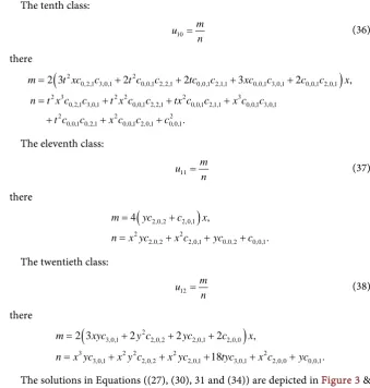
[image:11.595.198.538.75.432.2]

The solutions in Equations ((27), (30), 31 and (34)) are depicted in Figure 3 & Figure 4, respectively.

4. The N-Soliton Solutions of the (2 + 1)-Dimensional BLMP

Equation

Consider the N-soliton solutions of Equation (4) by using the perturbation ap-

[image:11.595.120.541.518.710.2]

[image:12.595.98.540.63.273.2]

Figure 4. Pictures of (31) with t = 1:3d plot (left) and Pictures of (34) with y = 1:3d plot (right).

proach and the Hirota direct method. Equation (6) is the bilinear form of Equa-tion (4) by using transformaEqua-tion 2 ln

(

)

x

u= − F . Expand the F into small pa-rameter exponential as follows

2 3

1 2 3

1 ,

F = +εf +ε f +ε f +

(39)

and λ =0.

Substituting Equation (39) into Equation (6) and comparing the coefficients of the same powers of ε give rise to

, 0,1 1

exp ,

N N

ij i j j j

i j j

i j

F A

µ µ = > µ µ =µ µ

 

=  + 

 

∑

∑

∑

(40)

where

(

)

(

)

(

)

(

)

33

2

, .

2

A_ij j i j i i

j j j j

i j i j i j

l l w w k kj

k x l y w t e

l l w w k k

η = + + = −  − + − 

 

+ _ + + + _

When ε =1, the one-soliton solution and two-soliton solution as follows. 1) One-soliton solution

1 1

1 , , ,

F = +f f =eη η=kx+ +ly wt where the coefficient k l w, , satisfy with 3

0,

lw k l+ = the one-soliton solution is

(

)

2 2

2 ln sech .

2 2

xx k

u= F = η (41) 2) Two-soliton solution

1 2

1 2 12

1 2 1 2

1 , , ,A

F = + +f f f =eη +eη f =eη η+ + where

1 k x l y1 1 w t1, 2 k x l y2 2 w t2 ,

η = + + η = + +

(

)

(

)

(

)

(

)

12

3

2 1 1 2 1 2

3

1 2 1 2 1 2

2

. 2

A l l w w k k

e

l l w w k k

 

− _ − + − _

=

 

+ _ + + + _

There, coefficients k l w_i, ,_{i i} 1, 2

(

i=

)

satisfy with l wi i+k li i3 =0, the two-soliton solution is

(

)

(

1 2

)

2 ln _xx 2 ln 1 .

xx

[image:13.595.64.543.66.244.2]

Figure 5. The resonance solution to Equation (4) with the parameters k1=0.4,k2= −0.6,l1= =l2 1, (left) indicates t=0, and (right) indicates t=220.

Figure 6. The resonance solution to Equation (42) with the parameters k1=0.4, 0.6, 1.5, 2,k2= − l1= l2= (left) indicates

240,

t= − (middle) indicates t=0 and (right) indicates t=240.

When the coefficient eAij =0, the soliton solution is changed into the reson-ance solution. Its propagation will be showed in Figure 5.

Let the coefficient eAij ≠0, the two-soliton happen in the collision because of the different soliton speed. The pursue collision between the two soliton will be showed in Figure 6.

5. Conclusion

With the help of the generalized bilinear methods [9] [11] [12] [15], we present the bilinear form to the (2 + 1)-dimensional BLMP equation and the (2 + 1)-dimensional BLMP-like equation. Afterwards, the twelve classes of rational so-lutions are obtained respectively. The 3d graphics to the rational soso-lutions shows some properties about these rational solutions, such as symmetry. These rational solutions which can be described as a kind of algebraic solitary waves have great potential in applied value in atmosphere and ocean. Every solitary wave velocity is different (the faster speed wave will overtake the slower speed wave), so it comes to a conclusion that these solutions are changed into the resonance solution when the coefficient eAij =0, and the soliton collision will happen when the coefficient

0 Aij

[image:13.595.61.542.291.404.2]

pre-vious speed and the direction. The generalized bilinear method could be applied to more high dimensional equation to obtain its rational solutions and deduce new equation. This method also could be applied to the half a discrete nonlinear diffe-rential equation and discrete nonlinear diffediffe-rential equation. Continuing to study this generalized bilinear method in depth is meaningful and interesting.

Acknowledgements

This work was supported by National Natural Science Foundation of China (No.11271007, No.61402265), Open Fund of the Key Laboratory of Ocean Circu-lation and Waves, Chinese Academy of Sciences (No.KLOCAW1401), Graduate Innovation Foundation from Shandong University of Science and Technology (No.SDKDYC170226) and Young Teachers Support Program of SDUST. These supports are greatly appreciated.

References

[1] Alzaidy, J.F. (2012) Exact Traveling Wave Solutions of Nonlinear PDEs in Mathemat-ical Physics. Applied Mathematics, 3, 738-745.

https://doi.org/10.4236/am.2012.37109

[2] Yang, B., Zhang, W.G. and Zhang, H.Q. (2014) Generalized Darboux Transformation and Rational Soliton Solutions for Chen-Lee-Liu Equation. Applied Mathematics and Computation, 242, 863-876.

[3] Nezhad, S., Sofla, M.Z. and Kavitha, L. (2014) New Rational Solutions for Relativistic Discrete Toda Lattice System. Communications in Theoretical Physics, 62, 363-372.

https://doi.org/10.1088/0253-6102/62/3/13

[4] Yang, H.W., Yin, B.S. and Shi, Y.L. (2012) Forced Dissipative Boussinesq Equation for Solitary Waves Excited by Unstable Topography. Nonlinear Dynamics, 70, 1389-1396.

https://doi.org/10.1007/s11071-012-0541-9

[5] Zhang, N. and Xia, T.C. (2015) A Hierarchy of Lattice Soliton Equations Associated with a New Discrete Eigenvalue Problem and Darboux Transformations. Internation-al JournInternation-al of Nonlinear Sciences and NumericInternation-al Simulation, 16, 301-306.

https://doi.org/10.1515/ijnsns-2014-0119

[6] Hirota, R. (2009) A Direct Method of Soliton Theory. Tsinghua University Press, Bei-jing.

[7] Li, Y.S. (1999) Soliton and Integrable System. Shanghai Scientific and Technological Education Publishing House, Shanghai.

[8] Chen, D.Y. (2006) An Introduction to Soliton. Science Press, Beijing.

[9] Zhang, Y.F. and Ma, W.X. (2015) A Study on Rational Solutions to a KP-Like Equa-tion. Zeitschrift für Naturforschung A, 70, 263-268.

https://doi.org/10.1515/zna-2014-0361

[10] Kudryashov, N.A. (2010) Soliton, Rational and Special Solutions of the Korteweg-De Vries Hierarchy. Applied Mathematics and Computation, 217, 1774-1779.

[11] Zhang, Y. and Ma, W.X. (2015) Rational Solutions to a KdV-Like Equation. Applied Mathematics and Computation, 256, 252-256.

[12] Ma, W.X. (2011) Generalized Bilinear Differential Equations. International Journal of Nonlinear Sciences, 2, 140-144.

Communications in Theoretical Physics, 63, 401-405.

https://doi.org/10.1088/0253-6102/63/4/401

[14] Hirota, R. (1971) Exact Solution of the Korteweg-De Vries Equation for Multiple Col-lisions of Solitons. Physical Review Letters, 27, 1192-1194.

https://doi.org/10.1103/PhysRevLett.27.1192

[15] Ma, W.X. and Xia, T.C. (2014) A Generalization of the Wadati-Konno-Ichikawa Soli-ton Hierarchy and Its Liouville Integrability. International Journal of Nonlinear Sciences and Numerical Simulation,15, 397-404.

https://doi.org/10.1515/ijnsns-2014-0013

[16] Dong, H.H., Zhang, Y.F. and Yin, B.S. (2014) Generalized Bilinear Differential Oper-ators, Binary Bell Polynomials, and Exact Periodic Wave Solution of Boi-ti-Leon-Manna-Pempinelli Equation. Abstract and Applied Analysis, 2014, 1-6.

https://doi.org/10.1155/2014/356350

[17] Gilson, C.R., Nimmo, J.J.C. and Willox, R. (1993) A (2 + 1)-Dimensional Generaliza-tion of the AKNS Shallow Water Wave EquaGeneraliza-tion. Physics Letters A, 180, 337-345. [18] Qu, C.Z. (1996) Symmetry Algebras of Generalized (2 + 1)-Dimensional KdV

Equa-tion. Communications in Theoretical Physics, 25, 369-372.

https://doi.org/10.1088/0253-6102/25/3/369

[19] Ma, W.X. (2011) Comment on the (3 + 1)-Dimensional Kadomtsev- Petviashvili Equ-ations.Communications in Nonlinear Science, 16, 2663-2666.

[20] Fu, H.W., Song, Y. and Xu, J. (2012) Wronskian and Grammian Solutions for Genera-lized (n + 1)-Dimensional KP Equation with Variable Coefficients. Applied Mathe-matics, 3, 154-157. https://doi.org/10.4236/am.2012.32024

[21] Wazwaz, A.M. (2013) Two B-type Kadomtsev-Petviashvili Equations of (2 + 1) and (3 + 1) Dimensions: Multiple Soliton Solutions, Rational Solutions and Periodic Solu-tions. Computers & Fluids, 86, 357-362.

[22] Yue, C. and Xia, T.C. (2014) Algebro-Geometric Solutions for the Complex Shar-ma-Tasso-Olver Hierarchy. Journal of Mathematical Physics, 55, 249-315.

https://doi.org/10.1063/1.4891605

[23] Yu, F.J. and Yan, Z.Y. (2014) New Rogue Waves and Dark-Bright Soliton Solutions for a Coupled Nonlinear Schrodinger Equation with Variable Coefficients. Applied Mathematics and Computation, 233, 351-358.

[24] Kharif, C., Pelinovsky, E. and Slunyaev, A. (2009) Rogue Waves in the Ocean. Sprin-ger-Verlag, Berlin.

[25] Song, L.L., Chen, W., Xu, Z.H. and Chen, H.L. (2015) Rogue Wave for the Benjamin Ono Equation. Advances in Pure Mathematics, 5, 82-87.

https://doi.org/10.4236/apm.2015.52010

[26] Nather, H. and Abdullah, F.A. (2012) The Basic (G'/G)-Expansion Method for the Fourth Order Boussinesq Equation. Applied Mathematics, 3, 1144-1152.

https://doi.org/10.4236/am.2012.310168

[27] Li, Z.B. (2008) Travelling Wave Solutions of Nonlinear Mathematical Physics Equa-tions. Science and technology press, Beijing.

Submit or recommend next manuscript to SCIRP and we will provide best service for you:

Accepting pre-submission inquiries through Email, Facebook, LinkedIn, Twitter, etc. A wide selection of journals (inclusive of 9 subjects, more than 200 journals)

Providing 24-hour high-quality service User-friendly online submission system Fair and swift peer-review system

Efficient typesetting and proofreading procedure

Display of the result of downloads and visits, as well as the number of cited articles Maximum dissemination of your research work

Submit your manuscript at: http://papersubmission.scirp.org/