Munich Personal RePEc Archive
Evaluating Case-based Decision Theory:
Predicting Empirical Patterns of Human
Classification Learning (Extensions)
Pape, Andreas and Kurtz, Kenneth
Binghamton University (SUNY)
18 March 2013
Evaluating Case-based Decision Theory: Predicting Empirical Patterns of
Human Classification Learning (Extensions)
Andreas Duus Papea,1,∗, Kenneth J. Kurtzb
a
Economics Department, Binghamton University, PO Box 6000, Binghamton NY, 13902
b
Psychology Department, Binghamton University, PO Box 6000, Binghamton NY, 13902
Abstract
We introduce a computer program which calculates an agent’s optimal behavior according to Case-based Decision Theory (Gilboa and Schmeidler, 1995) and use it to test CBDT against a benchmark set of problems from the psychological literature on human classification learning (Shepard et al., 1961). This allows us to evaluate the efficacy of CBDT as an account of human decision-making on this set of problems.
We find: (1) The choice behavior of this program (and therefore Case-based Decision Theory) correctly predicts the empirically observed relative difficulty of problems and speed of learning in human data. (2) ‘Similarity’ (how CBDT decision makers extrapolate from memory) is decreasing in vector distance, consis-tent with evidence in psychology (Shepard, 1987). (3) The best-fitting parameters suggest humans aspire to an 80−85% success rate, and humans may increase their aspiration level during the experiment. (4) Average similarity is rejected in favor of additive similarity.
JEL codes: D83, C63, C88
Keywords: Case-based Decision Theory, Human Cognition, Learning, Agent-based Computational
Economics, Psychology, Cognitive Science
1. Introduction
We present a computational implementation of Case-based Decision Theory (Gilboa and Schmeidler, 1995) called the Case-based Software Agent or CBSA. CBSA is a computer program that calculates an agent’s optimal behavior according to Case-based Decision Theory for an arbitrary problem. Like Expected Utility Theory, Case-based Decision Theory is a mathematical model of choice under uncertainty. Case-based Decision Theory has the following primitives: A set ofproblems or circumstances that the agent faces; a set
ofactions that the agent can choose in response to these problems; and a set ofresults which occur when an
action is applied to a problem. Together, a problem, action, and result triplet is called acase, and can be thought of as one complete learning experience. The agent has a finite set of cases, called amemory, which it consults when making new decisions.
∗Corresponding author
Email addresses: [email protected](Andreas Duus Pape),[email protected](Kenneth J. Kurtz) 1
The Case-based Software Agent is asoftware agent, i.e. “an encapsulated piece of software that includes data together with behavioral methods that act on these data (Tesfatsion, 2006).” CBSA computes choice data consistent with an instance of CBDT for an arbitrary choice problem or game, provided that the problem is well-defined and sufficiently bounded (see Section 3). To examine CBSA’s relationship with human learning, we chose to generate data for a set of problems from the psychological literature on human classification learning starting with Shepard et al. (1961). In these problems, human decision makers classify objects described by vectors of characteristics, such as color and shape, and are rewarded when they classify the objects correctly. The data include variables such as probability of error over time, which allows one to observe relative difficulty and speed of problem-solving/learning. We generate simulated choice data that is both consistent with Case-based Decision Theory and directly comparable to human data collected on the same set of problems.
This is the first instance of simulating nuanced choice data implied by an economic decision theory that can be brought to existing human choice data from psychology. Behavioral economics is typically characterized by applying insights from psychology to economics via a mathematical model, sometimes with modification, which is then tested using economic statistical methodologies on economic data (e.g. Laibson (1997), Fudenberg and Levine (2006)). This paper does the reverse: it tests a decision theory from economics using psychological methods and data.
In the framework of Case-based Decision Theory, the effects of actions on new problems are extrapolated from memory by evaluating thesimilarity between problems. The extrapolation from problems in CBDT is similar to generalization from stimuli in psychology. The study of generalization in psychology has lead to a remarkably specific empirical estimate of the functional form of similarity among humans (Shepard, 1987). We test this form with CBSA and find empirical support.
We are able to establish four key facts about CBDT and its relationship with human choice behavior in these classification learning experiments.
First, we find the choice behavior of CBSA fits two canonical experiments’ worth of human choice data very well. The best-fitting benchmark model fits both the relative difficulty of these categorization problems and the speed of learning to solve these sorting problems (i.e. probability of error over time). Moreover, the best-fitting benchmark model fits human data with a mean-squared error near the leading choice models in psychology. (This is the standard that psychology uses to evaluate models of classification learning.) This consistency with human behavior should be taken as a vote of confidence in support of CBSA as an account of human decision-making.2
Second, we find that, consistent with research in psychology cited above (Shepard, 1987), similarity functions that are decreasing in vector distance induce the best match to human data. On the other hand, whether the distance is mapped to similarity via an inverse exponential function, versus some other decreasing function, appears to not be critical.
Third, we find the best-fitting aspiration level, which can be thought of as a target success rate in the
2This is an account of human decision-making in the same sense that a representation theorem provides an account of
classification problem, is 80−85%. This falls into the range consistent with a correctly-specified choice model.3 We also find some evidence that agents start at a lower aspiration level, around 70%, and increase their aspiration levels during the course of the experiment in a manner consistent with Gilboa and Schmeidler (1996).
Fourth, we find that additive similarity provides a better match for human data than does average similarity.
We augment CBDT in two ways in this computational implementation. First, we provide a dynamic, endogenous similarity function following the ALCOVE model from psychology (Kruschke, 1992). A dynamic similarity function is necessary to match one of the two human data sets; the other is matched with static similarity. Second, we introduce two different models of imperfect memory: imperfect storage (stochastic ‘writing to memory’) and imperfect recall (stochastic ‘reading from memory’). Imperfect memory brings the speed of CBSA problem mastery in line with humans: with perfect memory, CBSA learns much too fast. Moreover, it appears that imperfect recall is more important than imperfect storage, which suggests cognitive processing limitations as opposed to storage-capacity limitations.
Below, we review the relevant literature in decision theory and agent-based computational economics (Section 2); we define CBSA precisely, then show that CBSA correctly and completely implements Case-based Decision Theory (CBDT), and therefore an instance of CBSA is an instance of CBDT (Section 3); we then introduce the psychology of human classification learning and relate it to decision theory (Section 4), including defining the two augmentations of CBDT we pursue (Subsections 3.3 and 4.3). Then we present and discuss our empirical results (Section 5) and conclude with some implications for future work (Section 6).
2. Related Literature
To define a decision theory in the tradition of Savage and von Neumann and Morgenstern, an agent’s choice behavior is observed and, if the choice behavior follows certain axioms, then a mathematical represen-tation of utility, beliefs, et cetera can be constructed (von Neumann and Morgenstern, 1944; Savage, 1954). In an implementation, this is turned on its head: the mathematical representation is taken as given and choice behavior is produced. The purpose is to generate choice behavior for particular problems in hopes of finding empirical patterns in choice behavior that were not be a priori obvious from the mathematical representation alone. These patterns, coupled with human choice data, can be used to empirically test the hypothesis that the implemented decision theory describes human behavior. We do that here.
Case-based Decision Theory (Gilboa and Schmeidler, 1995)—hereafter, CBDT—postulates that when an agent is confronted with a new problem, she asks herself: How similar is today’s case to cases in memory? What acts were taken in those cases? What were results? She then forecasts payoffs of actions using her memory, and choses the action with the highest forecasted payoff.
Formally, in CBDT, the following objects are taken as primitives: (1) a finite set of problems P, (2) a set of resultsRor outcomes, and (3) a finite set of actsAwhich interact with problems to form results. A
3Unless the model is misspecified, the aspiration level must lie between 50%, which is achievable by random selection, and
set of casesC is definedC =P × A × R, and a subset of casesM⊆ C will be called the “memory” of this agent. The memory is the data set that the agent draws on to make decisions.
Gilboa and Schmeidler (1996) define two functions: “utility” and “similarity.” Utility u : R → R
measures desirability. Similaritys:P × P →[0,1] represents how similar one decision problem is to another. Together, they define case-based utility as:
CBU(a) = X
(q,a,r)∈M(a)
s(p, q) [u(r)−H]
WhereM(a) is defined as the subset of the agents’ memoryMin which action awas taken, andH ∈Ris an aspiration level (see below). This utility represents the agent’s preference in the sense that, for a fixed memoryM,ais strictly preferred toa′ if and only ifCBU(a)> CBU(a′).
CBDT requires an aspiration levelH, which the agent uses as a default value for forecasting utility of new alternatives. “Behaviorially,Hdefines a level of utility beyond which the DM does not appear to experiment with new alternatives”(Gilboa and Schmeidler, 1996, page 2). In the experiment considered in this paper, the aspiration level has a natural interpretation: it is the target success rate in the classification problem.
This paper contributes to a small literature empirically testing the explanatory power of case-based decision theory; like this paper, these papers find support for CBDT. Gayer et al. (2007) investigate whether case-based reasoning appears to explain human decision-making using housing sales and rental data. They hypothesize and find that that sales data are better explained by rules-based measures because sales are an investment for eventual resale and rules are easier to communicate, while rental data are better explained by case-based measures because rentals are a pure consumption good where communication of measures are irrelevant. This is consistent with our results. Ossadnik et al. (2012) run a repeated choice experiment involving unknown proportions of colored and numbered balls in urns. They find that CBDT explains these data well compared to alternatives such as minimax (Luce and Raiffa, 1957) and reinforcement learning (Roth and Erev, 1995). Golosnoy and Okhrin (2008) investigate using CBDT to construct investment portfolios from real returns data and compare the success of these portfolios to investment portfolios constructed from EUT-based methods, and find some evidence that using CBDT aids portfolio success.
The central investigative tool of this paper is asoftware agent, which is “an encapsulated piece of software that includes data together with behavioral methods that act on these data (Tesfatsion, 2006).” CBSA is thus part of Agent-based Computational Economics. In fact, CBSA is the first example of agent-based computational economics making a direct contribution to decision theory. Software agents are common in the field of artificial intelligence, which, like decision theory, also cites von Neumann as a founder. The fields are largely distinct, with some notable exceptions, such as Gilboa and Schmeidler (2000), who describe how CBDT is “closely related to (and partly inspired by) the theory of Case-Based Reasoning proposed by Riesbeck and Schank (1989) and Schank (1986).”
CBSA is written in the agent-based modeling platform NetLogo (Wilensky, 1999).
3. Case-based Software Agent Description and Verification
Gilboa and Schmeidler (1996). First we describe the primitives of the implementation. Then we describe the algorithms, which implement CBDT in this setting (as we argue in Section 3.2). Finally, we extend the implementation to handle imperfect memory (Section 3.3).
3.1. Primitives of the Implementation
This implementation has three types of primitives: first, the primitives of CBDT; second, the CBDT representation; third, a decision environment.
The primitives and representation of CBDT define aspects of decision-making internal to the agent. The primitives of CBDT are: a finite set of actionsA, a finite set of problemsP, a set of resultsR, and the set of casesC =P × A × R.Moreover, a set M⊆ C is memory of this agent. From the CBDT representation, the agent is also endowed with a similarity function s : P × P → R+ and a utility function u: R → R. The similarity value is interpreted as: the higher a similarity values(p, q), the more relevant is problemqto problempin the mind of the decision-maker.
The decision environment defines those aspects of the series of problems the agent faces that are external to the agent. We capture the decision environment with a function (algorithm) called theproblem-result map
or P RM. TheP RM is the transition function of the environment. It takes as input the current problem
p∈ Pthe agent is facing, the actiona∈ Athat the agent has chosen, and some vectorθ∈Θ of environmental characteristics. TheP RM returns the outcome of these three inputs: namely, it returns a resultr∈ R; the next problemp′∈ Pthat the agent faces; and a potentially modified vector of environmental characteristics
θ′ ∈Θ.I.e.:
P RM :P × A ×Θ→ R × P ×Θ
For example, consider the canonical Savage omelette problem (Savage, 1954, pp. 13-15): the agent must choose to crack an egg in the main or secondary bowl, and the egg may be rotten or good. The acts are Main or Secondary. A particular egg is a problem, and the similarity function could describe visual clues about eggs. Now consider a series of Savage omelette problems. The P RM can be thought of as a device which delivers new eggs to the agent. It provides an egg which is rotten or not (which embeds the result of each action) and maintains aθ which describes the remaining eggs.
TheP RMwhich corresponds to the classification learning problem from psychology is specified in Section 4.2.2.
3.2. Algorithms of the Implementation
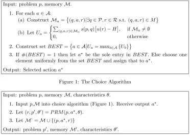
Figure 1 describes the choice algorithm which implements the core of CBDT. The agent faces a problem
p∈ P and has a memoryM⊆ C. For each actiona that she has available to her, she consults her memory and collects those cases, Ma, in which she performed this act. Then she uses this subset of her memory
to construct a cumulative utility of that act, called here Ua. This value is a similarity-weighted payoff: a sum across the cases in Ma, the result times the similarity between the problem faced at that time and
the current problem. The agent then chooses the action which corresponds to the maximumU.There is an additional step, left unspecified in the original CBDT: In the case of a tie, the agent randomizes uniformly over the acts which achieve this maximum.
Input: problemp, memoryM.
1. For eacha∈ A: (a) ConstructMa=
(q, a, r)|∃q∈ P, r∈ Rs.t. (q, a, r)∈M
(b) LetUa =
(P
(q,a,r)∈Mas(p, q)
u(r)−H
, ifMa6=∅
0, otherwise
2. Construct set BEST =
a∈ A
Ua = maxb∈A{Ub}
3. If #(BEST) = 1 then let a⋆ be the sole entry in BEST. Else choose one
element uniformly from the setBEST and assign that toa⋆.
[image:7.612.120.492.71.343.2]Output: Selected actiona⋆
Figure 1: The Choice Algorithm
Input: problemp, memoryM, characteristicsθ.
1. Inputp,Minto choice algorithm (Figure 1). Receive outputa⋆.
2. Let (r, p′, θ′) =P RM(p, a⋆, θ).
3. LetM’ =M ∪ {(p, a⋆, r)}
[image:7.612.127.492.75.201.2]Output: problemp′, memoryM′, characteristicsθ′.
Figure 2: A Single Choice Problem.
decision making, the algorithm described in Figure 2 embeds the agent in an environment and explicitly references that environment, in the call toP RM.In step one, the agent selects an act,a⋆.In step two, the
action is performed, in the sense that the environment of the agent reacts to the agent’s choice: the P RM
takes the current problem p, the actiona⋆ selected by the agent, and the characteristics unobserved by the
agentθ,and constructs a resultr, a next problemp′, and a next set of characteristicsθ′. In step three, the agent’s memory is augmented by the new case which was just encountered: that is, the case that was just experienced is added to the set M. Note that the choice problem maps a problem, characteristic, memory vector to another vector in the same space, so it can be applied iteratively.
1. InitializeM=∅. Initializeθ.Initialize first problemp.
2. Evaluate single choice problem with input (p,M, θ). Receive output (p′,M′, θ′).
3. Evaluate: Does (p′, θ′) achieve ending condition? If so, stop. Else, return to
previous step with new vector (p′,M′, θ′)
Figure 3: A Complete Series of Choice Problems.
Figure 3 describes a complete series of problems faced by an agent. Initially, the agent is assumed to have an empty memory, and some initial problem p.4 Furthermore, it is assumed that there is some initial starting conditionθ.Essentially, thereafter, the single choice problem is repeated iteratively. In step three
4
p′ andθ′ are jointly evaluated against some ending condition, and if that ending condition is achieved, the
algorithm halts.
3.3. Extending the Implementation to Imperfect memory
In the experimental results (Section 5), we demonstrate that the computational implementation of CBDT described until now masters the problems in these experiments much quicker than humans. To bring our implementation closer in line with human data without resorting to irrational behavior such as a trembling hand, we implement imperfect memory.5 There are two ways we consider incorporating imperfect memory into this model.
Method one: imperfect storage. In this method, we addpstore, which is a probability that any given event is stored in memory; after a case is experienced by an agent, there is simply a (1−pstore) probability that the case is immediately forgotten. Formally, this causes a modification to the algorithm depicted in Figure 2, step 3. The modification is depicted in Figure 4.
3’) With probabilitypstore, LetM’ =M ∪ {(p, a⋆, r)} Else letM’ =M
Figure 4: Modification to Figure 2 due to Stochastic Storage
Method two: imperfect recall. Instead of a probability that any given case is stored, the probability that a given event is accessed or recalled is less than one. We call this probabilityprecall. Formally, when finding the subset of memory that is relevant to a new problemp, in step 1a of the algorithm depicted in Figure 1, we draw a binary random variable for each case in memory, and include that case when the binary variable is 1. The modification due to stochastic recall is depicted in Figure 5.
1a’) For each (q, a, r)∈ M, draw r.v. b(q,a,r)=
(
1, with probabilityprecall 0 otherwise.
ConstructMa=
(q, a, r)|b(q,a,r)= 1 AND∃q∈ P, r∈ Rs.t. (q, a, r)∈ M
Figure 5: Modification to Figure 1 due to Stochastic Recall
Imperfect storage would imply that the relevant limitation is memory space. Imperfect recall would imply that the relevant limitation is cognitive capacity. There is some evidence from psychology that imperfect recall should be the preferred choice: the brain exhibits activity during each trial, which suggests every trial is somehow encoded. We evaluate these two theories of memory in explaining human data in Section 5, and find some support for the view that imperfect recall is more important.
4. Psychology of Human Classification Learning
The classification problem is used regularly in psychology and cognitive science to study both natural and artificial agents (Pothos and Wills, 2011). The classification learning problem presents a standard set
of objects to the agent, who must classify the objects in categories. The correct classifications vary in complexity and are therefore harder or easier to learn. Psychologists have collected data on how humans solve these problems. These data include variables such as probability of errors over time. Psychologists have also developed a number of Models of Classification Learning (MCLs), which, like CBSA, are mathematical models that are implemented as software programs to generate simulated choice data. Psychologists compare the fit of MCLs to human data to evaluate the MCLs’ explanatory power. We evaluate CBSA in the same way to establish our central results.
Game theorists might describe the classification problem as: a choice problem of sorting a series of vectors into bins, where Nature provides a true mapping of vectors to bins, and the agent’s utility is determined by her accuracy in following Nature’s mapping. Savage’s omelette problem (Savage, 1954, pp. 13-15) can be considered a classification problem.
4.1. The SHJ Classification Experiment
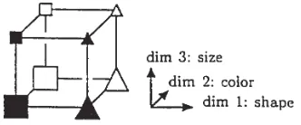
[image:9.612.220.386.370.439.2]Shepard et al. (1961) performed a canonical laboratory experiment which established some empirical facts about human classification learning. In this study, Shepard et al. (1961) (hereafter SHJ) introduced a set of objects to be classified: eight elementary objects with three binary dimensions of shape (square or triangle), color (dark or light), size (large or small). These eight objects can be thought of as three-digit binary strings. Figure 6 is an illustration of these objects as they are typically represented in the psychology literature: each binary string is placed on a vertex of the unit cube. SHJ also introduced a now standard
Figure 6: The eight elementary objects introduced by SHJ.
(Image from Nosofsky et al. (1994).)
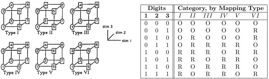
set of mappings or classifications T ={I, II, . . . , V I}. SHJ named the six mappings “Problems of Type I
throughV I.” It is the relative and absolute performance of sorting under each of these six mappings that we measure here. Figure 7 shows the six mappings graphically and as a table, where each of the eight objects is represented as three-digit binary string. Category one is represented by ovals (the letter O) and category two is represented by rectangles (the letter R).
In the Type I mapping, only the first dimension, e.g. shape, is required to sort the objects correctly: the left face of the first cube is marked with ovals and the right face is marked with rectangles. By contrast, in the relatively complicated TypeV I mapping, all three dimensions are required to sort the objects correctly. The intuition that Type VI is more complicated than Type I is reflected in human performance. In repeated trials, humans learn Type I problems much faster than Type VI.6 In these trials, images of these eight objects were shown to people in a laboratory setting in a random order, and, after each category guess,
6There are several empirical facts that have been established about orderings of the Problem TypesI throughV I. See
Digits Category, by Mapping Type 1 2 3 I II III IV V V I
0 0 0 O O O O O O
0 0 1 O O O O O R
0 1 0 O R O O O R
0 1 1 O R R R R O
1 0 0 R R R O R R
1 0 1 R R O R R O
1 1 0 R O R R R O
[image:10.612.86.529.71.201.2]1 1 1 R O R R O R
Figure 7: Classifications of Type I through IV.
(Image from Nosofsky et al. (1994).)
the subjects were told whether or not they were correct and given the correct label. MCLs are put through the same process and given the same feedback. Whether MCLs achieve the same ordering over problems is an important metric of success in explaining human data in the psychology literature, and it is a metric we use here (see Section 5).
4.2. Classification Learning and Case-based Decision Theory
The purpose of this section is to interpret the classification learning problem as understood and tested by psychologists into the Case-based Decision Theory/CBSA framework, in order to ‘run’ CBDT on the classification problem in a way to generate simulated data comparable to human data and those simulated data generated by other MCLs. After relating some fundamental concepts in the psychology of classification learning to decision theory, we formally define the the problem-result map (PRM) consistent with the SHJ series of classification learning experiments and choose a functional form of similarity based on empirical work in psychology. (We test this functional form of similarity against alternatives.)
4.2.1. Related concepts in Psychology and Decision Theory
The concept of aproblemin CBDT corresponds to the concept of astimulusin psychology. In describing the classification learning experiment, a psychologist would refer to an object shown to a decision-maker as a stimulus. Accordingly, the concept of the problem set P corresponds to the psychological concept of
a psychological space. Psychologists impose more structure on a psychological space than does CBDT on
a problem set: A psychological space is assumed to be an n-dimensional space, in which each dimension represents some characteristic of the stimuli. By contrast, the problem space in CBDT need not have any particular structure. In SHJ, since the objects have three dimensions, the psychological space is a subset of
R3. Since the dimensions are binary, the unit cube is the psychological space of the classification problem. This is why psychologists chose to represent the eight three-digit binary strings to the vertices of a cube (as seen in Figure 6). It also implies that a natural sense of similarity be based on geometric distance.
(Shepard, 1987). Case-based Decision Theory describes one way humans might generalize.
4.2.2. The Problem-Result Map (PRM) implied by the Classification Learning Experiments
The Problem-Result Map, or PRM (see Section 3), takes as input {an action a∈ A, a problem p∈ P, and a set of environmental characteristicsθ ∈Θ,} and delivers{a result in r∈ R, a ‘next problem’ p′ the
agent is to face, and a potentially modified vector of environmental characteristicsθ′∈Θ}. In this section,
we define the primitives of CBDT needed to describe the classification problem introduced by SHJ and then define the PRM.
We define the primitives as follows: Let P be the complete set of three-digit binary strings (therefore #(P) = 23= 8). Let A={a
1=O, a2=R} be the set of categories. There is a correct mapping, given by
Nature, from stringsp∈ Pto categoriesa∈ AcalledF :P → A. Each mappingF is called aclassification, and someFs may be harder to learn than others. We useFI throughFV Ito evaluate CBSA; these mappings correspond to the SHJ “Problems of Type I through VI” described above. There is also an aspiration level
H which can be thought of as the target success rate.
Briefly, the choice problem proceeds as follows: Nature selects a stringp∈ Pand presentspto the agent. The agent observes p, and announces a category guessa⋆ ∈ A. Her payoff is determined by whether her
guess is correct, and then Nature presents the agent with a new problemp′.
The environmental characteristic θ ∈ Θ describes those aspects of the environment that are changing over time. In the classification problem, the only aspect of the environment that is changing over time is the randomization device: i.e. how Nature determines the next binary string p∈ P that will be encountered. We assume that Nature selectsp∈ Paccording to some distribution; we let Θ be the set of all distributions overP, so at any given point in time, the next problem will be selected according to the current distribution
θ∈Θ.
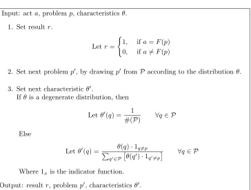
The PRM in Figure 8 describes how the environment responds to the agent choice.
In Step 1, the result ris determined in the following way: ifa⋆=F(p), then the agent’s category guess
matches the true category for that string, and his answer is ‘correct,’ and r = 1. If a⋆ 6=F(p), then the
guess is ‘incorrect’ and the agent receives a payoff of 0. Given an aspiration levelH, then, the payoff that an agent receives is (1−H) in the case of a correct answer and−H in the case of an incorrect answer, so if the agent aspires to, for example, a 75% success rate, then the agent receives payoffs.25,−.75.
In Step 2, the next problemp′ is selected.
In Step 3, the next distribution is specified. We are not free to chooseθ′; instead, the series ofθs must correspond to how the problems/strings were selected in the actual SHJ experiments. The new environmental characteristic θ′ ∈ Θ is given by: if all the elements ofP have been selected, then θ′ is set to a uniform distribution overP.7 Otherwise, set to zero the probability of the problem just selected,p′, and reweight the
remaining probabilities according to Bayes’ Rule. This follows the procedure of SHJ, in which the objects were selected uniformly but without replacement.8
7Any distribution overPcould be substituted here, if desired. The uniform distribution is chosen to be consistent with the
human experiments. 8
This description is slightly simplified. For the interested reader, we describe the exact randomization process: The first
sixteen trials consist of: the first eight trials consist of all elements ofPin a random order, and the second eight trials are again,
all elements ofPin a random order. In the second set of sixteen trials, each element of set ofPis presented twice in a random
Input: acta, problemp, characteristicsθ.
1. Set result r.
Letr=
(
1, ifa=F(p) 0, ifa6=F(p)
2. Set next problemp′, by drawingp′ fromP according to the distributionθ.
3. Set next characteristic θ′.
Ifθ is a degenerate distribution, then
Letθ′(q) = 1
#(P) ∀q∈ P
Else
Letθ′(q) = P θ(q)·1q6=p q′∈P
θ(q′)·1
q′6=p
∀q∈ P
Where 1xis the indicator function.
[image:12.612.127.491.60.336.2]Output: resultr, problemp′, characteristicsθ′.
Figure 8: The Classification Learning PRM
4.2.3. The Functional Form of Similarity suggested by Psychology
Psychology has done a good deal of research about the functional form of similarity common to humans. Shepard (1987), in the journalScience, finds that “[e]mpirical results and theoretical derivations point toward two pervasive regularities of generalization.” He finds that similarity “approximates an exponential decay function of distance in psychological space.”
In the classification problem, the dimensionality and psychological space of the stimuli are carefully controlled. In this case, Shepard’s result has remarkably specific implications about the functional form of similarity: similarity ought to be measured by the inverse exponential of vector distance. Applying this result, our primary similarity function, which we call simplys, is:
s(p, q) = 1
ed(p,q) wherep, q∈ {0,1}3
andd(p, q) =
v u u t
3
X
i=1
h
αi(pi−qi)2i
andpi refers to the ith element ofp
andαi≥0, ∀i
The Euclidean distance is weighted with parametersαi, called ‘attentional weights.’ These weights reflect the relative importance of some dimensions relative to others.9 The initial value of these weights reflect the agents’ priors about the problem at its onset. In the SHJ problem, it would be natural to assume that all dimensions have equal prior weight: that is, a priori the agent should think there is no particular reason
that shape is more important than color. In psychology, it is thought that these attentional weights might
change over the course of a run for a particular agent, as the agent learns that some dimensions are more important for categorization than others. For example, in problem Type I, the only relevant dimension is the first. Presumably the agent could learn to increase the weight on the first dimension and lower the weights on the other two dimensions in that case. We consult the psychology literature for guidance on how to update these weights.
A well-known and successful model of human classification learning (Kruschke, 1992, ALCOVE)10 uses the same similarity function above11 and also provides a formula for updating attention weights.12 The formula adjusts the attentional weight “proportionally to the (negative of the) error gradient (p. 24, ibid).” We construct an update rule by translating the pieces of the ALCOVE update rule into CBSA. This is that rule:
Suppose a new casec′= (p′, a′, r′) just occurred and supposeM is the memory of this agent. Then ∆αi
is the change in attentional weightαi due to this new case.
Definexi =−λ X
(p,a,r)∈M h
s(p, p′)· pi−p′i
·(u(r′)−κ) i
Then let ∆αi =xi−
P ixi
# Dimensions
whereλandκare constants defined below.
Let us describe the intuition of each part of this equation:
λis a parameter which describes the speed of learning these weights. Whenλ= 0, there is no updating. Then we sum over each case in memory, three terms:
The first term represents how similar the problem in memory is to the current choice. If this number is small, then, all else equal, the change inαi due to this particular case (p, a, c) will be small.
The second term pi−p′i
captures how important dimension i is to the formulation of this choice. It
serves as a flag to indicate whether this dimension doesn’t match the current problem: only dimensions that do not match are updated.
The third term, (u(r′) +κ) represents whether the choice made was a good choice. κis chosen so that
u(r′)−κ >0 when it should be considered a ‘good choice.’ For example,κcould be the agent’s expected
value ofuorκcould be equal to the agent’s aspiration levelH. Here, we find the natural level ofκis.5, so that correct choices are valued at.5 and incorrect choices are valued at−.5.
9Billot et al. (2008) provide an axiomatic foundation to this functional form, including weighted Euclidean distance among
problems described as vectors. 10
We describe ALCOVE in more detail, and compare its results to CBSA, in Section 5.3. 11
Equation 1, p. 23 (ibid.)
The intuitive appeal of this formulation can be seen though an example. Suppose the agent just made a good choice, so (u(r′)−κ)>0. Suppose moreover that a particular problem pin memory is very similar to the current problemp′, sos(p, p′) is large. Now suppose that dimension idoesn’t match betweenpand
p′. One can conclude that dimension i is not as important to the decision as other dimensions. Since a ‘good choice’ was made, the agent concludes that dimensioni’s “unimportance” was correct, so the weight is reduced (note the negative sign.)
Now suppose the agent just made a bad choice, i.e. (u(r′)−κ)< 0. Again, suppose moreover that a particular problem pin memory is very similar to the current problem p′, sos(p, p′) is large and suppose
that dimensioni doesn’t match betweenpand p′. One can conclude that dimensioni is not as important to the decision. Since the decision was incorrect (because it was a bad choice) the agent concludes that i
“unimportance” wasincorrect, so the weight is increased (note the negative sign.) The final term, Pixi
# Dimensions, assures us that per-period changes sum to zero. This corrects for overall drift in the weights.
This is the similarity function we use to generate the primary results below. We test this form of similarity against others. These results are described in Section 5.2.
4.3. The stylized facts of SHJ and related experiments
Here we describe the core phenomenology or stylized facts of human classification learning that have been empirically established with the SHJ problem set. The original findings of Shepard et al. (1961) have been replicated using contemporary research methodology as a benchmark for comparison of formal models (Nosofsky et al., 1994).
I < II < III, IV, V < V I
The key findings are the ease of Type I learning, the difficulty of Type VI learning, approximately equal difficulty of Types III, IV, V, and a Type II advantage relative to Types III, IV, V. These results have been replicated repeatedly except for the Type II advantage which appears to depend on particular experimental conditions (Kurtz et al., 2012). Leading theoretical accounts suggest that this pattern of performance is attributable to some type of psychological mechanism that allows human learners to focus their attention on, verbalize, or abstract rules or regularities about particular dimensions (characteristics) of the stimuli.
are found between Types III, IV, and V. In addition, the learning is slower in general.
I < IV < III < V < II < V I
In its pure form, CBSA does not have a focusing mechanism, because the similarity is assumed to be fixed. Therefore, the appropriate human data with which to test ‘pure’ CBSA is the integral-stimuli benchmark Nosofsky and Palmeri (1996), called here NP96. On the other hand, the appropriate human data with which to test CBSA augmented with updating attention weights (see Section 4.2.3) is the human data in Nosofsky et al. (1994), called here N94. We show below in Section 5.1 that CBSA matches human data in this way: with attention weight updating, it best matches N94, and without, NP96.
5. Experimental Results
This section has two parts. In the first part, we consider a benchmark model, and in the second part we consider model variants. The purpose of the benchmark model is to present a version of CBSA which best fits the human data. The purpose of the variants is to evaluate alternative specifications.
When discussing fit to human data, there are two relevant human data sets that these models are compared to, N94 and NP96, which are described in detail in Section 4.1. The data are: probability of error
by block for each of the first twenty-five blocks, for each problem of problem TypeI throughV I, averaged across all human subjects. This provides a total of 150 data points (25 blocks ×6 Problem Types) for each experiment. They can each be thought of as a panel data set, where the panel is performance by Problem Type over time. The primary difference between N94 and NP96 is the objects that are to be classified. In N94, the eight objects have the dimensionsshape,color, andsize, which are easy to distinguish; In NP96 the eight objects have the dimensionshue, brightness, and saturation, which are hard. Given this difference, in N94, the expected behavior is that humans learn which dimensions are important. In NP96, the expected behavior is that humans do not learn which dimensions are important. As a consequence, the prediction made here is that the best-fit value of λ is greater than zero (some level of attention weight updating) in N94 and the best-fit value ofλis zero (no attention weight updating) in NP96.13
There are three considerations in choosing a benchmark model: qualitative fit, quantitative fit, and model complexity.
Qualitative fit to human data is equivalent to matching “stylized facts” of human data. For example, in N94, Problem Type V I is the most difficult problem (highest probability of error) in all 25 blocks, and simulation data that have this property are considered to have a better qualitative fit than those that do not. The more of these regularities are matched, the greater the qualitative fit.
Quantitative fit is a numeric evaluation of fit to human data: for any given set of simulated data, we construct mean squared error (MSE) between the simulation average probability of error by block and human averages of the same variable. The lower the MSE, the better the quantitative fit. Even though perfect quantitative fit implies perfect qualitative fit, in practice quantitative fit often comes at the cost of qualitative fit.
13
Model complexity is also known as overfitting in econometrics. This third consideration rests on the observation that if a model is allowed to be arbitrarily complicated, then perfect qualitative and quantitive fit can be achieved, but such a model may be undesirable because it doesn’t reveal insight into human learning and is not generalizable to other kinds of learning. The ‘model complexity’ consideration leads us to select a simpler model over a more complicated one.
Best-fitting models were chosen by exploring the parameter space through an iterated grid-search. That is: the parameter space was swept at a certain resolution, and the part of the parameter space that contained the best fitting models by the considerations listed above (particularly quantitative and qualitative fit) was then explored at a higher resolution. This was repeated several times until the MSE seemed to no longer improve except at a cost of qualitative fit. At each stage, each parameter combination was populated with 600 simulation runs.
5.1. The best-fitting benchmark model
The benchmark model has: (1) the inverse exponential of distance similarity function with potentially endogenous similarity “attention weights” as described in Section 4.2.3 and a parameterλfit to human data, (2) imperfect recall of memory as described in Section 3.3 with a parameter precall fit to human data, and (3) an aspiration success rate parameter H which is fit to human data. Because it contributes little to the effectiveness of the match to human data,pstore is considered a variant (see Section 5.2 below.)
0.0 0.1 0.2 0.3 0.4 0.5
1 2 3 4 5 6 7 8 9 10 11 12 13 14 15 16 17 18 19 20 21 22 23 24 25
[image:16.612.84.294.355.541.2]! ! ! !! ! ! ! ! ! ! !! ! ! ! ! ! !! ! ! ! ! ! ! ! ! ! ! ! ! ! ! ! ! ! ! ! ! ! ! ! ! ! ! ! ! ! ! I II III IV V VI ! !
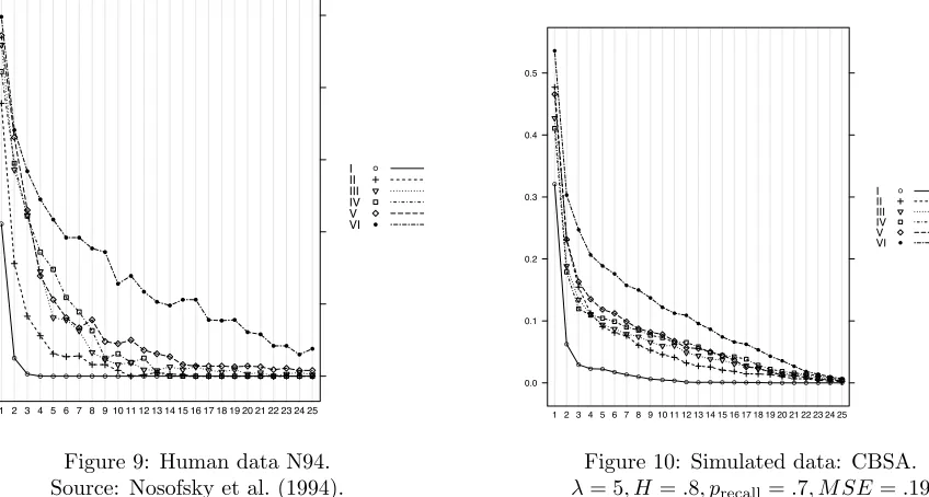
Figure 9: Human data N94. Source: Nosofsky et al. (1994).
0.0 0.1 0.2 0.3 0.4 0.5
1 2 3 4 5 6 7 8 9 10 11 12 13 14 15 16 17 18 19 20 21 22 23 24 25
[image:16.612.99.523.358.585.2]! ! !! !!!!! !!!!! !!!!! !!!!! ! ! ! ! ! ! ! ! ! ! ! !! ! ! ! !! ! ! ! ! !!! ! I II III IV V VI ! !
Figure 10: Simulated data: CBSA.
λ= 5, H =.8, precall=.7, M SE=.19
Best-fit benchmark model for N94.
Matching human data of SHJ’61 / Nosofsky et al ’94. The best-fitting benchmark model for N94 has a
MSE of.185, with aspiration level H =.8 and probability of recallprecall =.7. Qualitatively, the pictures in Figures 9 and 10 can be seen to display many of the same characteristics: the same general shape, the same approximate ordering ofI < II≤III, IV, V < V I. The CBSA simulated data exhibits some TypeII
V Iproblems appears to converge to others in the CBSA simulated data, which is not exhibited by humans. (It is worth noting that other MCLs in the psychology literature also display this convergence.)
λis found to be 5, which is, as hypothesized, strictly larger than zero; so the best-fitting model exhibits attention weight updating when the human subjects were able to separately perceive the dimensions of the objects.
If perfect memory is assumed then CBSA never makes more than ten mistakes, and never after the first sixteen trials. CBSA with perfect memory is orders of magnitude faster than humans on the same problem. Therefore, perfect memory can be rejected.
The best-fitting aspiration level isH =.8, which corresponds to agents aspiring to an 80% success rate, so the best-fitting aspiration level is within the reasonable range (i.e. between .5 and 1). A best-fitting aspiration level outside of that range would be a strike against the model.
A slightly better MSE of .16 can be achieved with with aspiration level H = .86 and probability of recallprecall=.75, but in those simulated data TypeII separation is not observed. Note that Kurtz et al. (2012) find that whether humans exhibit TypeIIseparation depends on the specification of the experimental description to the human subjects. So this alternative may in fact be a better fitting model to human data.
0.0 0.1 0.2 0.3 0.4 0.5
1 2 3 4 5 6 7 8 9 10 11 12 13 14 15 16 17 18 19 20 21 22 23 24 25
[image:17.612.83.293.307.502.2]! ! ! ! ! ! ! ! !! ! ! ! !! ! ! ! !! ! ! ! !! ! ! ! ! ! ! ! ! ! ! ! ! ! ! ! ! ! ! !! ! ! ! ! ! I II III IV V VI ! !
Figure 11: Human data NP96. Source: Nosofsky and Palmeri (1996).
0.0 0.1 0.2 0.3 0.4 0.5
1 2 3 4 5 6 7 8 9 10 11 12 13 14 15 16 17 18 19 20 21 22 23 24 25 ! ! ! ! ! ! ! ! !! ! ! ! ! !!!!!! !!!!! ! ! ! ! ! ! ! ! ! ! ! ! ! !! !! ! !! !! !!! I II III IV V VI ! !
Figure 12: Simulated data: CBSA.
λ= 0, H=.85, precall=.6, M SE=.17
Best-fit benchmark model for NP96.
Matching human data of Nosofsky and Palmeri 96. The best-fitting benchmark model for NP96 has an
MSE of.17, with an aspiration levelH =.85 and a probability of recallprecall=.8. The pictures in Figures 11 and 12 can also be seen to display many of the same characteristics: the same general shape, the same approximate ordering ofI < IV < III < V < II < V I. λis fitted to a value of zero, which conforms to the hypothesis; so the best-fitting model exhibits no attention weight updating when the human subjects were able to not separately perceive the dimensions of the objects.
[image:17.612.328.529.322.502.2]rejected.
5.2. Model Variants
In this section we investigate alternatives to the benchmark models in the previous section. CBDT as described in the economics literature allows for many possibilities that are not represented in the benchmark models above, so we would like to show that these alternatives do not provide better fits than the benchmark models.
Imperfect memory through imperfect storage. In the benchmark model, imperfect memory was
imple-mented through imperfect recall, not imperfect storage. We found that little was gained from implementing imperfect storage, so the model complexity consideration lead us to drop this fitted parameter from the model. In particular, we found the best fitting imperfect storage value was.95 in both N94 and NP96 with approximately equal MSE and a small increase inprecall. On the other hand, simulations in whichprecallwas constrained to equal 1 resulted in a much higher MSE (doubling) and results in the behavior that problem Type VI becomes easier than other problems around trial 4, which is behavior not exhibited by humans.
Functional form of similarity. Shepard (1987) recommends the inverse exponential of Euclidean distance
for matching human notions of similarity (i.e. e−d(p,q), where d(p, q) is Euclidean vector distance). The exponential functional form of distance appears not to be critical. We test against two alternatives to the inverse exponential function s recommended by Shepard. The two alternatives considered here are of a simple inverse and inverse log, which we calls′ ands′′ respectively:
s′(p, q) = 1
d(p, q) + 1 s
′′(
p, q) = 1
ln (d(p, q) + 1) + 1
(Ones are added to avoid division-by-zero and log-of-zero problems.) In these results, there is no difference in the relative difficulty ranking for N94 and NP96 and a similar quantitative fit is achieved.
In contrast, it is critical that similarity decreases in geometric distance. The underlying distance met-ric dictates which objects the agent extrapolates (or generalizes) to first. To understand this, consider the similarity function s=, in which all objects are similar to themselves but all other objects are equally dissimilar.
s=(p, q) =
1 ifp=q
0 otherwise su(p, q) =
1 ifp=q
.5 otherwise
Unders=, an agent does not extrapolate from any object to any other object. A minor variant, su, can be thought of as a uniform prior, in which all distinct objects are thought to be equally similar. Under both of these distance metrics, the agent finds problems of Type I through VI to be equally difficult. This clearly conflicts with human data.14 In addition, one can also find similarity functions which are organized around principles other than geometric distance, which can reverse orderings consistent in all human data (N94
14
Curiously, the similarity functions=delivers a learning rate that matches human learning with the same memory parameter
values (precall=.7) at par with learning the easiest problem (TypeI), and also beats the functionsu. This suggests that
and NP96). For example, one similarity function induces agents to find problem TypeV I, consistently the hardest in human data, easier than problem TypeI, which is consistently the easiest in human data.15
0.0 0.2 0.4 0.6
1 2 3 4 5 6 7 8 9 10111213141516171819202122232425
[image:19.612.113.266.116.312.2]● ● ●● ● ●● ●● ● ● ● ● ●● ●●● ●●● ●● ●● ● ● ● ● ● ● ● ● ● ●● ● ● ● ● ● ● ● ● ● ● ● ● ● ● ● ● ●●● ● ● ● ● ● ● ● ●●● ● ● ● ● ● ● ● ●● ● ● ● ● ●● ● ● ● ● ● ● ● ● ● ● ● ● ● ● ● ● ● ● ● ● ● ●● ● ● ● ● ●● ● ● ● ●● ● ● ●● ● ●●● ●● ● ● ● ● ● ● ● ● ● ● ●● ● ● ● ● ● ● ● ● ● ● ● ● ● ● ● ● ●●● ● ● ● ● ● ● ● ●●● ● ● ● ● ● ● ● ●● ● ● ● ● ● ● ● ● ●● ● ●● ● ● ● ● ● ● ●●● ● ● ● ● ●● ● ● ● ● ● ● ● ● ● ● ● ● ● ● ● ● ● ● ● ● ●● ●
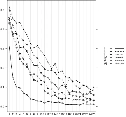
Figure 13: Random Sample of Runs, CBSA Additive Similarity, Category VI
0.0 0.2 0.4 0.6
1 2 3 4 5 6 7 8 9 10111213141516171819202122232425
! ! ! ! ! ! ! !! ! ! !! !!! !! !!! !!!! ! ! ! ! ! ! ! ! !! ! ! ! ! !! ! ! ! !! ! ! ! ! ! ! !!! ! ! ! !!! ! ! ! ! ! ! ! ! ! !! ! ! ! ! ! ! !! ! ! ! ! ! ! ! !! ! ! ! ! ! !!! ! ! ! ! ! ! !!! ! ! ! ! ! ! ! ! !! ! ! ! ! ! !! ! ! ! !!!!! ! ! ! ! ! !! ! ! ! !! ! ! ! !! ! ! ! ! ! ! ! ! ! ! ! ! ! ! ! !! ! ! ! ! ! ! ! ! ! !
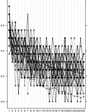
Figure 14: Random Sample of Runs, CBSA Average Similarity Variant, Category VI
Average similarity is an alternative similarity function proposed in Gilboa and Schmeidler (1995). It has
the following functional form:
savg(p, q) = P s(p, q)
(q′,a,r)∈Ms(p, q′)
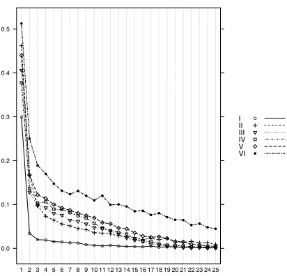
Normal similarity, also called additive similarity, accumulates weight with similarity and data accumulation. Average similarity removes the data accumulation aspect. The qualitative and quantitative fit of average similarity simulations are approximately the same as the benchmark model. This suggests that additive versus average similarity may be unimportant. However, a closer inspection of the simulated data reveals this is not true. Figure 13 depicts thirty randomly-selected runs of the best-fitting benchmark model, considering only the behavior on the Problem Type VI.16 The mean value for all runs and the human data are also depicted. Note that the simulated data forms something of a cloud around the mean. Figure 14 depicts thirty randomly-selected runs of the model with average similarity. In this figure, most of the simulated data also form something of a cloud around the mean; however, a small number of cases hover around a probability of error of .5. Closer inspection of these runs reveals that this .5 probability of error
15
The similarity function in question, called heres+is:
s+(p, q) = 1
2
P3
i=1pi−P3j=1qj +d(p, q)
wheredis Euclidean distance. This is a similarity function that declares vectors are more similar when their entries sum to the
same number; i.e. it judges (1,1,0) as fairly similar to (0,1,1), because their entries both sum to 2.
16
[image:19.612.367.514.125.313.2]results from the agent choosing the same category for all objects: in these cases, the agent acts as if one of the action strictly dominates the other. This single-action behavior seems inconsistent with human behavior.
Input: aspiration valueH, memoryM
Parameters: Mix probabilityp1, mix levelα1, Base increase probabilityp2, increase amountγ2
1. Mix with long run average: With probabilityp1,
H′= (1−α1)H+α1
P
(q,a,r)∈Mr
#(M)
!
Else
H′=H
2. Occasionally increase aspiration level: With probability p2
#(M)
H′′=H′+γ2
Else
H′′=H′
[image:20.612.120.492.108.368.2]Output: New aspiration valueH′′
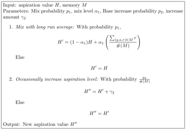
Figure 15: The Aspiration Updating Algorithm
A dynamic, endogenous aspiration level can assure long-run convergence to optimal behavior in repeated
choice settings such as this one, provided the updating scheme that is ‘ambitious’ and ‘realistic’ (Gilboa and Schmeidler, 1996). That is, an aspiration level that starts below the long-run average payoff, updates to the long-run average payoff in some mixture with the current level, and also occasionally receives increases that are unrelated to the relationship between the aspiration level and long-run average payoff. Moreover, these increases must happen decreasingly often, and converge to occur with a probability of zero. We implement this scheme in this framework as depicted in Figure 15. Note that the rate of convergence diminishes at a rate proportional to the number of trials; this rate could also be considered another parameter.
Although this method does not improve the fit for NP96, it does appear to make a qualitative improvement for N94; see Figures 16 and 17. TypeII separation is seen earlier than in the benchmark model, and problem typeV Iremains more difficult than the other problems through the final block. A value of p1=.03 means that updating to the average occurs about once every two blocks ( 1
2·16 ≈.03) and a value ofp2 =.06 and
γ2 =.1 means that the aspiration level increases approximately once every block, by .1 each time.17 The MSE, at.22, remains comparable to the benchmark model. Therefore, among the variations considered here, the strongest argument could be made for this variation; only the model complexity criterion argues against it.
0.0 0.1 0.2 0.3 0.4 0.5
1 2 3 4 5 6 7 8 9 10 11 12 13 14 15 16 17 18 19 20 21 22 23 24 25
[image:21.612.84.294.73.269.2]! ! ! !! ! ! ! ! ! ! !! ! ! ! ! ! !! ! ! ! ! ! ! ! ! ! ! ! ! ! ! ! ! ! ! ! ! ! ! ! ! ! ! ! ! ! ! I II III IV V VI ! !
Figure 16: Human data. Source: N94. 0.0 0.1 0.2 0.3 0.4 0.5
1 2 3 4 5 6 7 8 9 10 11 12 13 14 15 16 17 18 19 20 21 22 23 24 25 ! ! ! !! ! ! !! ! !! ! ! !! ! !! ! ! !! ! ! ! ! ! ! ! ! ! ! ! ! ! ! ! ! !! ! ! ! ! ! !! ! ! I II III IV V VI ! !
Figure 17: CBSA w/ endogenous aspiration level
λ= 6.5, precall=.7,Initial H=.7, M SE=.22
p1=.03, α1=.2, p2=.06, γ2=.1
5.3. Comparison to Cognitive Models
One leading formal model of classification learning is known as ALCOVE (Kruschke, 1992). ALCOVE is one of only a handful of computational models that provide a good fit to N94, and it is the only one that has been shown, like CBSA, to also fit NP96. ALCOVE is an adaptive network model (artificial neural network) that instantiates the exemplar theory of categorization (Medin and Schaffer, 1978; Nosofsky, 1986). The exemplar view states that the psychological representation of a category is the stored examples themselves (i.e., no abstractions are formed) and the process of classification is based on the similarity between each stored example and the stimulus. The trial-by-trial learning process in ALCOVE consists of storing each new object that is experienced and using error-driven learning to optimize both the mapping between examples and the correct category labels and attention weights for each dimension in the similarity function. By contrast, CBSA and CBDT store every trial, whether or not that trial involves encountering a new object.18 ALCOVE is able to match the N94 data on the same qualitative metrics as CBSA. ALCOVE also exhibits more pronounced TypeII separation. On quantitative fit, ALCOVE is substantially better: an MSE of.06 versus.17 for CBSA.19 ALCOVE is also able to match the NP96 data on all qualitative metrics, as CBSA has, with a MSE of.10 versus.17 for CBSA.
ALCOVE employs four free parameters: the rate of learning of association weights, the rate of learning of attention weights, the degree of specificity with which exemplars are activated by similar stimuli, and a bias on the mapping between category label activation and actual response behavior. When these parameter settings are optimized to match human data, high attentional learning and high specificity allow ALCOVE to best fit N94, while low (zero) attentional learning and low specificity produce a close fit for NP96 (Nosofsky
18
One might say that CBDT stores “task exemplars” to ALCOVE’s “object exemplars.”
19Nosofsky et. al report the mean squared error for the first sixteen blocks; the CBSA value reported here is also measured
[image:21.612.338.544.74.272.2]et al., 1994; Nosofsky and Palmeri, 1996). When CBSA’s parameters are optimized to match human data, CBSA also exhibits high attentional learning (λ >0) in N94 and low attentional learning (λ= 0) in NP96. In contrast to ALCOVE, however, the other parameters of the best fit are quite similar between the best fitting models ofN94 andN P96: H =.8, .85 andprecall=.7, .6. In fact, there is a single set of parameters
H =.825, precall=.65, andλ= 0,5 as appropriate, which fit both N94 and NP96 fairly well: with an MSE of.24 for N94 and.23 for NP96.
6. Conclusion
We present a computational implementation of Case-based Decision Theory (Gilboa and Schmeidler, 1995) that can generate choice data consistent with an instance of CBDT for an arbitrary choice problem. The implementation is called the Case-based Software Agent or CBSA. We use CBSA to test the performance on a benchmark set of problems from the psychological literature on human classification learning exemplified by Shepard et al. (1961) and Nosofsky et al. (1994). We find the choice behavior of CBSA (and therefore Case-based Decision Theory) fits two canonical experiments’ worth of human choice data very well. The best-fitting benchmark model fits both the relative difficulty of these categorization problems and the speed of learning to solve these classification problems (i.e. probability of error over time). We find that imperfect memory is an important factor to match human data: with perfect memory, CBDT learns the problem orders of magnitude faster than humans. On the topic of imperfect memory, we find some evidence that imperfect recall, instead of imperfect storage, is the mechanism that best matches human data. We find dimensionality of the problem is an important factor, and encoding the dimensionality according to their natural definition provides the best fit to human data. We find that the aspiration level is important: the best-fitting model indicates that humans aspire to a success rate between .8 and .85 on this problem, and they may increase their aspiration level during the experiment.
References
Billot, A., Gilboa, I., Schmeidler, D., 2008. Axiomatization of an exponential similarity function. Mathemat-ical Social Sciences 55 (2), 107–115.
Fudenberg, D., Levine, D., 2006. A Dual-Self Model of Impulse Control. The American Economic Review 96 (5), 1449–1476.
Gayer, G., Gilboa, I., Lieberman, O., 2007. Rule-based and case-based reasoning in housing prices. The B.E. Journal of Theoretical Economics (Advances) 7 (1).
Gilboa, I., Schmeidler, D., August 1995. Case-Based Decision Theory. The Quarterly Journal of Economics 110 (3), 605–39.
Gilboa, I., Schmeidler, D., 1996. Case-based Optimization. Games and Economic Behavior 15, 1–26.
Gilboa, I., Schmeidler, D., March 2000. Case-Based Knowledge and Induction. IEEE Transactions on Sys-tems, Man, and Cybernetics—Part A: Systems and Humans 30 (2), 85–95.
Golosnoy, V., Okhrin, Y., 2008. General uncertainty in portfolio selection: A case-based decision approach. Journal of Economic Behavior & Organization 67 (3), 718–734.
Kruschke, J., 1992. ALCOVE: an Exemplar-Based Connectionist Model of Category Learning. Psychological Review 99 (1), 22.
Kurtz, K. J., Levering, K., Romero, J., Stanton, R. D., Morris, S. N., 2012. Human Learning of Elemental Category Structures: Revising the Classic Result of Shepard, Hovland, and Jenkins (1961). Journal of Experimental Psychology: Learning, Memory, and Cognition, Forthcoming.
Laibson, D., 1997. Golden Eggs and Hyperbolic Discounting. The Quarterly Journal of Economics 112 (2), 443–477.
Luce, R. D., Raiffa, H., 1957. Games and Decisions. WIley, New York.
Medin, D., Schaffer, M., 1978. Context Theory of Classification Learning. Psychological Review 85, 207–238.
Nosofsky, R., 1986. Attention, Similarity, and the Identification–Categorization Relationship. Journal of Experimental Psychology: General 115 (1), 39–57.
Nosofsky, R., Gluck, M., Palmeri, T., McKinley, S., Glauthier, P., 1994. Comparing Models of Rule-Based Classification Learning: a Replication and Extension of Shepard, Hovland, and Jenkins (1961). Memory and Cognition 22, 352–352.
Nosofsky, R., Palmeri, T., 1996. Learning to Classify Integral-Dimension Stimuli. Psychonomic Bulletin and Review 3, 222–226.
Ossadnik, W., Wilmsmann, D., Niemann, B., 2012. Experimental evidence on case-based decision theory. Theory and Decision, 1–22.
Pothos, E., Wills, A., 2011. Formal Approaches in Categorization. Cambridge University Press.
Riesbeck, C. K., Schank, R. C., 1989. Inside Case-Based Reasoning. Lawrence Erlbaum Assoc., Hillsdale, NJ.
Roth, A. E., Erev, I., 1995. Learning in extensive-form games: Experimental data and simple dynamic models in the intermediate term. Games and Economic Behavior 8 (1), 164–212.
Savage, L. J., 1954. The Foundations of Statistics. Wiley.
Schank, R. C., 1986. Explanation Patterns: Understanding Mechanically and Creatively. Lawrence Erlbaum Assoc., Hillsdale, NJ.
Shepard, R., 1987. Toward a Universal Law of Generalization for Psychological Science. Science 237 (4820), 1317.
Shepard, R., Chang, J., 1963. Stimulus Generalization in the Learning of Classifications. Journal of Experi-mental Psychology 65 (1), 94–102.
Shepard, R., Hovland, C., Jenkins, H., 1961. Learning and Memorization of Classifications. Psychological Monographs 75, 1–41.
Tesfatsion, L., 2006. Handbook of Computational Economics. Vol. 2. Elsevier B.V., Ch. 16.
von Neumann, J., Morgenstern, O., 1944. Theory of Games and Economic Behavior. Princeton University Press, Princeton, NJ.
Wilensky, U., 1999. NetLogo.