Robust standard error estimators for panel models: a unifying approach

Robust standard error estimators for

panel models: a unifying approach

Millo, Giovanni

Research and Development, Generali SpA

7 July 2014

Models: A Unifying Approach

Giovanni Millo

Research and Development, Generali SpA

Abstract

The different robust estimators for the standard errors of panel models used in applied econometric practice can all be written and computed as combinations of the same simple building blocks. A framework based on high-level wrapper functions for most common usage and basic computational elements to be combined at will, coupling user-friendliness with flexibility, is integrated in the plm package for panel data econometrics in R_. Sta-tistical motivation and computational approach are reviewed, and applied examples are provided.

Keywords: Panel data, Covariance matrix estimators, R_.

1. Introduction

The so-called robust approach to model diagnostics, which relaxes the hypothesis of ho-moskedastic and independent errors from the beginning, has long made its way in Econo-metrics textbooks. Moulton (1986, 1990) has famously raised awareness about the perils of “clustering” inside a sample: observations belonging to the same cluster share common characteristics, violating the independence assumption and potentially biasing inference. In particular, variance estimates derived under the random sampling assumption are typically biased downwards, possibly leading to false significance of model parameters.

Although clustering can often be an issue in cross-sectional data too, it is an obvious feature in panels: the group (firm, individual, country) and the time dimension define natural clusters; observations sharing a common individual unit, or year, are likely to share common characters. The implications on inference are well known and studied; nevertheless, recent reviews in the finance (Petersen 2009) and in the accounting literature (Gow, Ormazabal, and Taylor 2010) highlight how a majority of papers in the respective disciplines still employ standard error estimators which are inconsistent even under reasonably mild departures from the classical hypothesis of homoskedastic and uncorrelated errors. In political science, as Wilson and Butler (2007) note, one particular “robust” method (Beck and Katz 1995) has effectively displaced all alternatives, overshadowing different potential sources of bias which are seldom taken into account.

GAUSS_orMATLAB_{code is available as well; estimators which are commonly preferred in one}

or the other branch of applied econometrics, from large microeconometric panels (Arellano 1987) to moderately-sized panel time series in macroeconomics (Driscoll and Kraay 1998) and large panels in finance (Petersen 2009;Cameron, Gelbach, and Miller 2011;Thompson 2011), up to pooled time series in political science (Beck and Katz 1995); all under the common umbrella of theR_{environment (R Development Core Team 2012), once again the all-purpose}

statistical software.

From a software design viewpoint, I translate some results from the recent literature (Petersen 2009;Thompson 2011;Cameronet al.2011) into a comprehensive computational framework, in turn integrated into the plm package for panel data econometrics (Croissant and Millo 2008). I describe a general expression for “clustering” estimators; then I review two-level clustering as a combination of simple clustering estimators and the extension to persistent effects by summation of lagged terms; lastly, I show how applying a weighting scheme to lagged covariance terms yieldsDriscoll and Kraay(1998)’s spatial correlation consistent (SCC) estimator (and, as a special case, that ofNewey and West 1987).

From an application perspective, I extend the treatment ofPetersen(2009) to double-clustering estimators plus time-persistent shocks as in Thompson (2011): a structure which, based on simulations inPetersen(2009), can be conjectured to successfully account for both individual effects and persistent idiosyncratic shocks. My approach also allows easy extension to a com-bination of effects which has not, to my knowledge, received attention in the literature yet: double-clustering as in Cameron et al. (2011) plus time-decaying correlation as in Driscoll and Kraay(1998). A practical example is given in Section 6.

One not-so-minor aim of this paper is to overcome sectoral barriers between different, if contiguous, disciplines: it is striking, for example, how few citations Driscoll and Kraay

(1998) on the panel generalization of theNewey and West(1987) estimator gets in the finance literature, especially in those papers that advocate what is essentially an unweighted version of their SCC covariance. Also,Arellano(1987) andFroot(1989), in the different contexts of fixed effects panels with serial correlation and of industry-clustered financial data, independently developed what is computationally the same estimator (referred in the following as one-way clustering) first described byLiang and Zeger(1986). Cross-referencing between the different branches of statistical and econometric research is still uncommon in this subject, to the point that raising awareness might be useful.1

From the point of view of political science, where panel – or time-series cross-section (TSCS) – data are an important methodological field, the functionality outlined here allows researchers to progress beyond the now-ubiquitous application of PCSE standard errors to pooled specifications, along the lines of Wilson and Butler (2007): both comparing it with alternative strategies and possibly combining it with individual effects, in order to tackle the all-important, and often overlooked, issue of individual heterogeneity (Wilson and Butler 2007, 2.2).

In this sense, my work is meant to provide R users with a comprehensive set of modular tools: lower level components, conceptually corresponding to the statistical “objects” involved, (see Zeileis 2006), and a higher-level set of “wrapper functions” corresponding to standard covariance estimators as they would be used in statistical packages: White heteroskedasticity-consistent, clustering, SCC and so on. Wrappers work by combining the same, few lower-level

1

components in multiple ways in the spirit of the Lego principle of Hothorn, Hornik, Van De Wiel, and Zeileis(2006), with obvious benefits for both flexibility and code maintenance. This toolset should enable users to follow the work ofPetersen(2009);Cameronet al.(2011);

Thompson(2011) in detail, experimenting with settings and comparing estimates’ magnitudes (seePetersen 2009) for specification and diagnostic purposes, at least as far as linear models in two panel dimensions are concerned. Extensions to multiple dimensions, which do not fit into the panel data infrastructure of packageplm, are left instead for future work.

When estimating regression models, R _{creates a model object which, besides estimation}

re-sults, carries on a wealth of useful information, including the original data. Robust testing inR _{is done retrieving the necessary elements from the model object, using them to}

calcu-late a robust covariance matrix for coefficient estimates and then feeding the latter to the actual test function, which can be a t-test for significance, a Wald restriction test and so on. Therefore the approach to diagnostic testing is more flexible than with procedural languages, where diagnostics usually come with standard output. In our case, for example, one can obtain different estimates of the standard errors under various kinds of dependence without re-estimating the model, and present them compactly.

When appropriate, I will highlight some features of R_{that make it easy and effective to}

com-bine statistical objects; in particular, functions as arguments; modularity and components reusing; function application over arrays of arbitrary dimension; and in general object orien-tation, which ensures application of the right method with the appropriate defaults for the object at hand through standard syntax.

The paper is organized into three main bodies. The next two Sections (2 and 3) review the statistical foundations of the methods and set the notation in terms of a few low-level compo-nents according to the Lego principle. The “Computational framework” Section 4, arguably the heart of the paper, describes the statistical building blocks in terms of computational objects characterized by a few standard “switches”, and their combinations in terms of user-friendly “wrapper” functions; then, in an object-oriented fashion, it discusses how and when it is (statistically) appropriate to apply the resulting user-level methods toplmobjects estimated in different ways: by either (pooled) ordinary least squares (OLS), fixed effects (FE), random effects (RE), or by first-differencing methods (FD). The remainder of the paper (Sections 5

and6) sets the new estimators in the context of theplmpackage and provides some examples of application.

1.1. Package version and installation

The functionality described here is available in plm since version 1.5-1.

Notice that as of this writing this version has not made it to the standard CRAN repository; it can instead be downloaded from R-Forge (www.r-forge.r-project.org). The latest version can be installed from withinR_{as follows:}

R> ## not run

R> # install.packages("plm", repos="http://R-Forge.R-project.org")

In this Section I briefly review the ideas behind robust covariance estimators of thesandwich

type, in order to provide a basis for the subsequent treatment of their panel extension. The reader is referred to any econometrics textbook, e.g.,Greene(2003) – on which this paragraph is based – for a formal treatment.

Consider a linear modely=Xβ+ǫand the OLS estimator ˆβOLS = (X⊤X)−1X⊤y. If one is interested in making inference on β, then an estimate ofV ar( ˆβ) is needed. If the error terms

ǫ are independent and identically distributed, then the covariance matrix takes the familiar textbook form: V ar( ˆβ) = ˆσ2

(X⊤_X)−1

, where ˆσ2

is an estimate of the error variance. This case is synthetically dubbedspherical errors, and the relative formulation ofV( ˆβOLS) is often referred to, somewhat inappropriately, as ”OLS covariance”2

.

Two approaches are possible if i.i.d. errors cannot be taken for granted, as is common in the mostly non-experimental contexts of econometrics. Either one tests for departures from these assumptions, and if none is rejected proceeds with the standard covariance (pre-testing ap-proach), or he uses a robust estimate of the covariance, allowing for departures from sphericity, in the first place (robust approach). Obviously, the success of a pre-testing strategy is depen-dent on the power properties of the screening tests employed, so that to stay on the safe side many practicing econometricians have got used to dropping the sphericity assumption alto-gether. It is in fact frequent these days, also in introductory textbook treatments (e.g.,Stock and Watson 2003) to relax the restrictive assumptions of independence and homoskedasticity in favour of robustness from the very beginning. Delving into the ongoing debate on which strategy to choose would be out of the purpose of this paper; suffice it here to say that the robust approach has gained popularity among statisticians, and especially econometricians, in recent times: for recommendations based on an extensive simulation exercise and a survey of practice dating back to the turn of the century seeLong and Ervin(2000).

Let us consider robust estimation in the context of the simple linear model outlined above. The problem at hand is to estimate the covariance matrix of the OLS estimator relaxing the assumptions of serial correlation and/or homoskedasticity without imposing any particular structure to the errors’ variance or interdependence.

As the estimator of the OLS parameters’ covariance matrix is

ˆ

V = 1

n( X⊤X

n )

−1

(1

nX

⊤_[σ2

Ω]X)(X ⊤_X

n )

−1

in order to consistently estimateV it is not necessary to estimate all then(n+ 1)/2 unknown elements in the Ω matrix but only theK(K+ 1)/2 ones in

1

n

n

X

i=1

n

X

j=1

σijxix⊤j

which may be called the meat of the sandwich, the two (X⊤_nX)−1

being the bread. (From now on, we will concentrate exclusively on the meat, and we will dispose of the 1/n terms throughout.) All that is required are pointwise consistent estimates of the errors, which is

2

The reason is that OLS is “best linear unbiased” (BLUE) under sphericity; yet this is confusing because other covariance estimators can be more appropriate for ˆβOLSunder different conditions. Notice that

satisfied by consistency of the estimator forβ (see Greene 2003). In the heteroskedasticity case, correlation between different observations is ruled out and themeat reduces to

S0=

1

n

n

X

i=1

σ_i2x_ix⊤_i

where the nunknownσ2

is can be substituted bye2i (see White 1980). In the serial correlation case, the natural estimation counterpart would be

1

n

n

X

i=1

n

X

j=1

eiejxix⊤j

but this structure proves too general to achieve convergence. Newey and West (1987) de-vise a (heteroskedasticity and-) autocorrelation consistent estimator that works based on the assumption of correlation dying out as the distance between observations increases. The Newey-West HAC estimator for themeat takes that of White and adds a sum of covariances between the different residuals, smoothed out by a kernel function giving weights decreasing with distance:

S0+

1

n

n

X

i=1

n

X

j=1

wletet−l(xtx⊤t−l+xt−lx⊤t)

withwl the weight from the kernel smoother, e.g., the Bartlett kernel function: wl= 1−_L+1l

(for a discussion of alternative kernels see Zeileis 2006)). The lag l is usually truncated well below sample size: one popular rule of thumb is L = n1/4

(see Greene 2003; Driscoll and Kraay 1998).

In the following I will consider the extensions of this framework for a panel data setting where, thanks to added dimensionality, various combinations of the two above structures will turn out to be able to accommodate very general types of dependence.

3. Clustering estimators in a panel setting

Let us now consider apanel (orlongitudinal) setting where data are collected on two different dimensions: to fix ideas, let us think of n entities (individuals, firms, countries...) which we here label groups and index by i = 1, . . . , n sampled at T points in time. The two dimensions are not fully symmetric as for the sake of practical relevance I have considered one dimension (time) having a natural ordering and the other having none. This setting is sufficiently general to describe the vast majority of applications; a symmetric extension would nevertheless be straightforward. Different choices of dimensions are possible and have been explored in the literature: e.g., Froot (1989), in the context of financial data, discusses sampling from ”independent” industries in order to increase sample size, clustering within industry to account for dependence. Thus the two dimensions would be industry and a generic counter: clustering would be done according to industry, while meaningless across the ”other” dimension. The model is then

For now I consider again the familiar OLS estimator ˆβOLS, which in this setting is referred to as pooled OLS because itpools all observations together irrespective of their belonging to a given group (but see Section 4.4for an extension to three other common panel estimators). Clustering estimators work by extending the ”sandwich” principle to panel data. Besides heteroskedasticity, the added dimensionality allows to obtain robustness against totally unre-stricted timewise or cross-sectional correlation, provided this is along the “smaller” dimension. In the case of ”large-N” (wide) panels, the big cross-sectional dimension allows robustness against serial correlation3

; in ”large-T” (long) panels, on the converse, robustness to cross-sectional correlation can be attained drawing on the large number of time periods observed. As a general rule, the estimator is asymptotic in the number of clusters.

Imposing cross-sectional (serial) independence in fact restricts all covariances between obser-vations belonging to different individuals (time periods) to zero, yielding an error covariance matrix with a block-diagonal structure: in the former case,V(ǫ) =In⊗Ωi, where

Ωi =

          σ2

i1 σi1,i2 . . . σi1,iT

σi2,i1 σ_i22 ...

..

. . .. ...

..

. σ2

iT−1 σiT−1,iT

σiT,i1 . . . σ_iT,iT−1 σ2_iT

          (1)

and the consistency relies on the cross-sectional dimension being ”large enough” with respect to the number of free covariance parameters in the diagonal blocks. The other case is symmetric.

3.1. White-Arellano, or one-way clustering

White’s heteroskedasticity-consistent covariance matrix4 _{has been extended to clustered data}

by Liang and Zeger (1986) and to econometric panel data by Arellano (1987), who applied it in a fixed effects setting. Observations can be clustered by the cross-sectional (group) index which is arguably the most popular use of this estimator, and is appropriate inlarge, short panels because it is based on n-asymptotics; or by the time index, which is based onT-asymptotics and therefore appropriate forlong panels. In the first case, the covariance estimator is robust against cross-sectional heteroskedasticity and also against serial correlation of arbitrary form. In the second case, symmetrically, against timewise heteroskedasticity and cross-sectional correlation. Arellano’s original estimator, an instance of the first case, has the form:

VW hite−Arellano= (X⊤X)−1 n

X

i=1

X_i⊤uiu⊤i Xi(X⊤X)−1 (2)

It is of course still feasible to rule out serial correlation and compute an estimator that is robust to heteroskedasticity only, based on the following error structure:

Ωi=

       σ2

i1 . . . 0

0 σ2

i2 ...

..

. . .. 0

0 . . . σ2

iT        (3) 3

This is the case of the seminal contribution byArellano(1987).

4

in which case the original White estimator applies:

VW hite= (X⊤X)−1 n X i=1 T X t=1

u2_itx_itx⊤_it(X⊤_X)−1 ₍₄₎

”White-Arellano”, or clustered, standard errors are popular in other areas of statistics, espe-cially afterRogers(1993) introduced them in the Stata software.

Some notation

Before discussing bidirectional extensions of this estimator, for the sake of clarity I will now define the ”meat” of the two versions of the Arellano estimator, henceforthVC., with respect to the clustering dimension: the original, group-clustered version, robust vs. heteroskedasticity andserial dependence, will be

VCX = n

X

i=1

X_i⊤uiu⊤i Xi (5)

while the time-clustered version, robust vs. heteroskedasticity andcross-sectionaldependence, will be:

VCT = T

X

t=1

X_t⊤utu⊤t Xt (6)

The standard White estimator on pooled data, which is symmetric w.r.t. clustering,

VW = T X t=1 n X i=1

u2_itx_itx⊤_{it (7)}

will be conveniently written as

VW = n

X

i=1

X_i⊤diag(u2_i)Xi = T

X

t=1

X_t⊤diag(u2_t)Xt (8)

wherediag(u2

) is a matrix with squares of elements ofuon the diagonal and zeros elsewhere, so that all of these expressions share the common structure

VC·=

X

·

X_·⊤E(u)X· (9)

withE(u) an appropriate function of the residuals.

This symmetric representation will provide a good starting point for the extension to double clustering.

3.2. Double clustering

Some recent research in finance (Petersen 2009;Cameronet al.2011;Thompson 2011) advo-cates double clustering, motivating it by the need to account forpersistent shocks and at the same time for cross-sectional or spatial correlation5

. The former case is more often dealt with

5

Spatial correlation is related to proximity in space, while cross-sectional correlation is more generally related to belonging to the same cross-section. An important class of data generating processes giving rise to cross-sectional dependence arecommon factor models, popular both in macroeconometrics and in finance (see

in the econometric literature by parametric estimation of random effects or serially correlated models, or, in a completely different theoretical specification, by inclusion of the lagged de-pendent variable, a strategy which is also popular in political science in the context of pooled time series models. The latter case has received attention in the spatial panel literature, where again it is estimated parametrically imposing a structure to the dependence, and in the common factor literature.

AsCameronet al.(2011) observe, though, double clustering, as all robustified inference of this kind, relies on much weaker assumptions as regards the data generating process than para-metric modelling of dependence does. In fact, this estimator combining both individual and time clustering relies on a combination of the asymptotics of each: the minimum number of clusters along the two dimensions must go to infinity. Apart from this, any dependence struc-ture is allowed within each group or within each time period, while cross-serial correlations between observations belonging to different groups and time periods are ruled out.

The double-clustered estimator is easily calculated by summing up the group-clustering and the time-clustering ones, then subtracting the standard White estimator (referred to in

Cameron et al. (2011) as time-group-clustering, in Thompson (2011) as white0) in order to avoid double-counting the error variances along the diagonal:6

VCXT =VCX+VCT −VW (10)

In order to control for the effect of common shocks,Thompson(2011) proposes to add to the sum of covariances one more term, related to the covariances between observations from any group at different points in time. Given a maximum lagL, this will be the sum overl= 1, ...L

of the following generic term:

VCT,l= T

X

t=1

X_t⊤utu⊤t−lXt−l (11)

representing the covariance between pairs of observations from any group distanced lperiods in time, summed with its transpose. As the correlation between observations belonging to thesame group at different points in time has already been captured by the group-clustering term, to avoid double counting one must subtract the within-groups part:

VW,l = T

X

t=1

n

X

i=1

[xituitu⊤i,t−lx⊤i,t−l] (12)

again summed with its transpose, for each l. The resulting estimator

VCXT,L=VCX +VCT −VW + L

X

l=1

[VCT,l+VCT,l⊤ ]− L

X

l=1

[VW,l+VW,l⊤ ] (13)

is robust to cross-sectional and timewise correlation inside, respectively, time periods and groups and to the cross-serial correlation between observations belonging to different groups,

6

up to the L-th lag. It also resembles another well-known estimator from the econometric liter-ature: the Newey-West nonparametric estimator, the difference being that instead of adding a (possibly truncated) sum of unweighted lag terms, the latter downweighs the correlation between “distant” terms through a kernel smoother function. Kernel-smoothed estimators will be the subject of the next Section.

3.3. Kernel-based smoothing

As cited above, in a time series contextNewey and West(1987) have proposed an estimator that is robust to serial correlation as well as to heteroskedasticity. This estimator, based on the hypothesis of the serial correlation dying out ”quickly enough”, takes into account the covariance between units by: weighting it through a kernel smoother function giving less weight as they get more distant; and adding it to the standard White estimator.

Driscoll and Kraay’s ”SCC”

Driscoll and Kraay (1998) have adapted the Newey-West estimator to a panel time series context, where not only serial correlation between residuals from the same individual in different time periods is taken into account, but also cross-serial correlation between different individuals in different times and, within the same period, cross-sectional correlation (see also

Arellano 2003).

The Driscoll and Kraay estimator, labeled SCC (as in ”spatial correlation consistent”), is defined as the time-clustering version of Arellano plus a sum of lagged covariance terms, weighted by a distance-decreasing kernel function wl:

VSCC,L = VCT +PLl=1wl[PTt=1Xt⊤utu⊤t−lXt−l+PTt=1[Xt⊤utu⊤t−lXt−l]⊤] = VCT +PLl=1wl[VCT,l+VCT,l⊤ ]

(14)

The “scc” covariance estimator requires the data to be a mixing sequence, i.e., roughly speaking, to have serial and cross-serial dependence dying out quickly enough with the T

dimension, which is therefore supposed to be fairly large: Driscoll and Kraay (1998), based on Montecarlo simulation, put the practical minimum at T > 20₋25; the n dimension is irrelevant in this respect and is allowed to grow at any rate relative toT.

Panel Newey-West

By restricting the cross-sectional and cross-serial correlation to zero one gets a ”pure” panel version of the original Newey-West estimator, as discussed, e.g., inPetersen(2009):

VN W,L = VW +PlL=1wl[PTt=1

Pn

i=1[xituitu⊤i,t−lx⊤i,t−l] +

PT

t=1[

Pn

i=1[xituitu⊤i,t−lx⊤i,t−l]⊤] = VW +PLl=1wl[VW,l+VW,l⊤ ]

(15) As is apparent from Equation 3.3.1, if the maximum lag order is set to 0 (no serial or cross-serial dependence is allowed) the SCC estimator reverts to the cross-section version (time-clustering) of the Arellano estimatorVCT. On the other hand, if the cross-serial terms are all unweighted (i.e., if wl= 1∀l) thenVSCC,L|w=1 =VCT,L.

Unconditional covariance estimators are based on the assumption of no error correlation in time (cross-section) and of an unrestricted but invariant correlation structure inside every cross-section (time period).7

They are popular in contexts characterized by relatively small samples, with prevalence of the time dimension. The most common use is on pooled time series, where the assumption of no serial correlation can be accommodated, for example, by adding lagged values of the dependent variable.

Beck and Katz PCSE

Beck and Katz (1995), in the context of political science models with moderate time and cross-sectional dimensions, introduced the so-called panel corrected standard errors (PCSE), an estimator with good small-sample properties which, in the original time-clustering setting, is robust against cross-sectional heteroskedasticity and correlation.8

In this framework and with reference to Equation9, the ”pcse” covariance is defined in terms of the Ei =E ∀ifunction of the residuals as:

E =

P

nˆetˆe⊤t

N

A sufficient, although not necessary condition for consistency of the “pcse” estimator (Beck and Katz 1996) is that the covariance matrix of the errors in every group be the same: Ω = Σ_⊗IT, with

Σ =           σ2

1 σ1,2 . . . σ1,T

σ2,1 σ22 ...

..

. . .. ...

..

. σ2

T−1 σT−1,T

σT,1 . . . σT,T−1 σ_T2

          (16)

A possible further restriction is to assume correlation away imposing that Σ be diagonal, thus restricting the estimator to unconditional intragroup heteroskedasticity.

4. Computational framework

Generalizing the computational problem at hand and dividing it into modules is necessary for writing software that be both full-featured and easy to read and to maintain. In this Section I show a generic formulation capable of generating all the estimators considered up

7

A further step in this direction is to use the unconditional estimate of the error covariance in a feasible GLS analysis: seeGreene(2003, p.322)Wooldridge(2002, p.263) and functionpggls in theplm package for

R; the original reference for FGLS isParks(1967).

8

Beck and Katz (1995) eloquently illustrate the shortcomings of the more general FGLS estimator of

Parks (1967), advocating their simpler solution. In particular, the fact that FGLS seriously understates variability “in practical research situations”, to a point which is not compensated by the increased precision of parameter estimates. This position, which has gained widespread acceptance in the political science field, is only justified whenever the sample sizes involved are at odds with the asymptotic properties of FGLS; otherwise an unrestricted GLS analysis is an attractive alternative (seeWooldridge 2002, 10.4.3). Noting how the overwhelming popularity of this approach has led to neglecting a number of other potential issues,Wilson and Butler(2007) have warned against simple prescriptions advocating the need for a more comprehensive specification approach. Recent simulations byChen, Lin, and Reed(2009) show that PCSE is actually less

to now; in the following I will consider a small-sample correction module. These building blocks will allow to construct a very general estimating function for a model’s parameters covariance whose usage in various testing environments will then be discussed in the light of object-oriented econometric computing.

Two defining features of R_{as a programming language are object-orientation and functional}

nature. In this sense, according to the object-oriented nature of R_{, in the next paragraph I}

will formulate a general computing module, thesoftware counterpart of thestatistical objects VW, VCX, VCT, VW,l, VCX,l and VCT,l which are in turn the building blocks for any of the estimators considered here. In turn, according to the functional nature of R_{, the computing}

module will be formulated as a function of: a (panel-indexed) vector of errors; an integer lag order; and lastly of a function to be applied to the error vector, taking the lag order as an argument. The ability of R_{to treat functions as a data type will make the translation of this}

formalization into software seamless.

4.1. A general, computing-oriented formulation

The most general formulation of the comprehensive estimator can be written as a kernel-weighted version of Formula 3 inThompson(2011):

VCXT,L|w =VCT + L

X

l=1

wl[VCT,l+VCT,l⊤ ] +VCX −VW − L

X

l=1

wl[VW,l+VW,l⊤ ] (17)

In turn, all building blocks for Formula 17 can be generated by combining a clustering di-mension, a function of the errors and a lag order. Starting from the general formulation:

Vg(t, l, f) = T

X

t=1

X_t⊤f(ut, ut−l)Xt−l (18)

inserting the outer product function and setting the lag to zero (so thatf(ut, ut−l) =utu⊤t ) we get the time- (group-) clustering estimator

VCT =Vg(t,0, f =utu⊤t ) (19)

and for the “White” terms on the diagonal

VW =Vg(·,0, f =diag(u2·)) (20)

while for the cross-serial terms

VCT,l=Vg(t, l, f =utu⊤t−l) (21)

and for the purely autoregressive ones:

VW,l =Vg(t, l, f =diag(ut×ut−l)) (22)

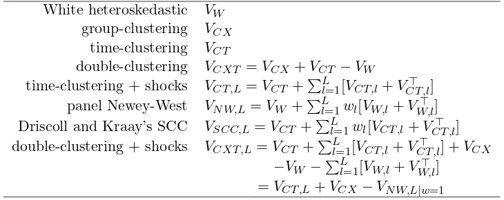
(where_×is the element-by-element product) so that by a (possibly weighted) combination of the above we can get all relevant estimators: see Table1.

White heteroskedastic VW group-clustering VCX

time-clustering VCT

double-clustering VCXT =VCX+VCT −VW

time-clustering + shocks VCT,L=VCT +PlL=1[VCT,l+VCT,l⊤ ] panel Newey-West VN W,L=VW +PLl=1wl[VW,l+VW,l⊤ ] Driscoll and Kraay’s SCC VSCC,L=VCT +PLl=1wl[VCT,l+VCT,l⊤ ] double-clustering + shocks VCXT,L=VCT +PLl=1[VCT,l+VCT,l⊤ ] +VCX

−VW −PLl=1[VW,l+VW,l⊤ ] =VCT,L+VCX−VN W,L|w=1

Table 1: Covariance structures as combinations of the basic building blocks.

Obviously, as there is no natural univariate ordering between individuals, a full generalization encompassing both the double-clustering and a two-way SCC estimator does not seem sensible. For the same reason, while the software components allow fully symmetric operation, i.e., it would be practically feasible to compute a group-clustering version ofVSCC,L orVCX,L, this is devoid of sense from a statistical viewpoint because the notion of a linear, unidimensional spatial lag is generally meaningless9

.

4.2. Unconditional estimation in the general framework

Unconditional estimators can also be computed from the general formulation by

precalculat-ing the unconditional error covarianceE =

PT t=1utu⊤t

T and substituting it inside the generic Formula (17) as a constant matrix:

VU T =Vg(t,0, f =E) (23)

One noteworthy feature of R is the ability to treat functions as first-class objects (R Develop-ment Core Team 2012), which means they are just another, although very special, data type and can be fed to another function as argument. So a function might indifferently take as argument a function or a precalculated matrix, which is the case here10

.

4.3. Unbalanced panels

Unbalancedness is one of the major computational nuisances in panel data econometrics. In the case at hand, the problem is to compute the generic Formula 17 taking heed that unbalanced samples will have incomplete groups (time periods) for somet(i). As the ultimate goal of estimation of themeat is to average the k_×k matrix productsX⊤

t f(ut, ut−l)X over time periods (or, symmetrically, groups), missing data will give rise to empty positions inXt and, correspondingly, inf(ut, ut−l).

9

Spatial lags, where applicable, are defined in a completely different way based on two-dimensional proximity matrices (seeAnselin 1988). One very special case of linear spatial arrangement allowing for a simple definition of lag isChudik, Pesaran, and Tosetti(2011)’s circular world, where each observation has one neighbour to the left and one to the right. Yet in that setting dependence would have to consider both directions, while serial dependence only originates from the past.

10

Fortunately, R has two particularly useful features for treating data in a ”generic” way, as independent as possible from dimensions: list objects and the apply family of functions. In general R makes it relatively easy to deal with unbalanced data through the use of structures likelists, very flexible containers which can hold e.g., matrices of different dimensions and on which operators (and, more generally,functions of any kind) can beapplied. Theapplyfamily has members for working member-by-member on lists (lapply), subgroup by subgroup on

ragged arrays (tapply) where (possibly heterogeneous) subgroups are defined by a grouping variable, or dimension by dimension on arrays, which is the original use ofapply. One notable advantage of this operator is that it can work on arbitrary subsets of the array’s dimensions, provided the function to be applied is compatible.11

If a function is applied that allows discarding of NA values, one can easily get consistent averaging over multidimensional arrays: in this case, an average of t k×k bidimensional matrices of uneven dimensions.

An example will clarify things. Let us take an array of three 3×3 matrices with a missing value, and average over the third dimension. By default, missing values propagate throughout operations:

R> a <- array(1, dim = c(3, 3, 3)) R> a[1, 1, 1] <- NA

R> apply(a, 1:2, mean)

[,1] [,2] [,3] [1,] NA 1 1

[2,] 1 1 1

[3,] 1 1 1

but the default behaviour can be overridden forcing discarding of NAs:

R> apply(a, 1:2, mean, na.rm = T)

[,1] [,2] [,3]

[1,] 1 1 1

[2,] 1 1 1

[3,] 1 1 1

In the latter case, the resulting 3_×3 matrix will contain all averages computed on the correct number of items (i.e., for the [1,1] position, (1 + 1)/2).

Analogously, in our case it will be convenient to make use of standard tridimensional arrays making a k_×k_×tmatrix – basically a ”pile” of X⊤

t f(ut, ut−l)X terms – and then applying themeanfunction over the third dimension, obtaining an appropriate calculation of Formula

17 as a result. In fact, for every value of t every product involving a missing element will

11

produce an NA in the relative k_×k matrix; but then averaging over the T dimension will discard NAs and apply the correct denominator.12

The same goes for the estimation of the unconditional covariance in Beck and Katz type estimators. This feature, which has been unavailable for unbalanced panels for a while and then has been twice mentioned in the literature as a potentially complicated computational problem (Franzese 1996; Bailey and Katz 2011) is solved nicely and without effort in R by applying (sic!) the above method, which acts as advocated by Franzese (1996), averaging elements in the unconditional covariance matrix on the correct number of observations13

.

4.4. Application to FE and RE models: The demeaning framework

The application of the above estimators to pooled data is always warranted, subject to the relevant assumptions mentioned before. In some, but not all cases, these can also be applied to random or fixed effects panel models, or models estimated on first-differenced data. The general idea is to use both the covariates and residuals from the transformed (partially or totally demeaned, first differenced) model used in estimation.

In all of these cases the estimator is computed as OLS on transformed data, e.g., in the fixed effects case ˆβF E = ( ˜X⊤X˜)−1X˜⊤y˜ with ˜yit = yit−yi. and ˜xjit = xjit−xji. for each xj in

X; while in the random effects case this time-demeaning is partial and ˜yit = yit−θyi. with 0 < θ < 1. Sandwich estimators can then be computed by applying the usual formula to the transformed data and residuals ˜u= ˜y₋X˜βˆ: see Arellano (1987) and Wooldridge (2002, 10.59) for the fixed effects case,Wooldridge (2002, Ch.10) in general.

Under fixed effects, the OLS estimator is biased and FE is required for consistency of param-eter estimates in the first place. Similarly, under the hypothesis of a unit root in the errors first differencing the data is warranted in order to revert to a stationary error term. On the contrary, under the random effects hypothesis OLS is still consistent, and asymptotically it makes no difference using RE instead. Yet for the sake of parameter covariance estimation it may be advisable to eliminate time-invariant heterogeneity first, by using one of the above. E.g., one compelling reason for combining a demeaning or a differencing estimator with robust standard errors may be to get rid of persistent individual effects before applying a more parsi-monious and efficient kernel-based covariance estimator if cross-serial correlation is suspected, or if the sample is simply not big enough to allow using double-clustering. In fact, asPetersen

(2009) shows, the Newey-west type estimators are biased if effects are persistent, because the kernel smoother unduly downweighs the covariance between faraway observations.

In the following I discuss when it is appropriate to apply clustering estimators to the residuals of demeaned or first-differenced models.

Fixed effects

The fixed effects estimator requires particular caution. In fact, under the hypothesis of spher-ical errors in the original model, the time-demeaning of data induces a serial correlation

cor(uit, ui,t−1) =−1/(T −1) in the demeaned residuals (see Wooldridge 2002, p.275).

12

Of course the most delicate programming issue becomes correct handling of the positions of incompleteut

subvectors andXt submatrices in the relevantt-th ”layer” of the tridimensional array.

13

The White-Arellano estimator has originally been devised for this case. By way of symmetry, it can be used for time-clustered data with time fixed effects. The combination of group-clustering with time fixed effects and the reverse seems inappropriate because of the serial (cross-sectional) correlation induced by the time- (cross-sectional-) demeaning.

By analogy, the Newey-West type estimators can be safely applied to models with individual fixed effects (for an application, seeGolden and Picci 2008), while the time and twoway cases require caution. The best policy in both cases, if the degrees of freedom allow it, is perhaps to explicitly add dummy variables to account for the fixed effects along the ”short” dimension.

Random effects

In the random effects case, asWooldridge(2002) notes, the quasi-time demeaning procedure removes the random effects reducing the model on transformed data to a pooled regression, thus preserving the properties of the White-type estimators.

By extension of this line of reasoning, all above estimators seem to be applicable to the demeaned data of a random effects model, provided the transformed errors meet the relevant assumptions.

First-differences

First-differencing, like fixed effects estimation, removes time-invariant effects. Roughly speak-ing, the choice between the two rests on the properties of the error term: if it is assumed to be well-behaved in the original data, then FE is the most efficient estimator and is to be preferred; if on the contrary the original errors are believed to behave as a random walk, then first-differencing the data will yield stationary and uncorrelated errors, and is therefore advisable (seeWooldridge 2002, p.281). Given this, FD estimation is nothing else than OLS on differenced data, and the usual clustering formula applies (seeWooldridge 2002, p.282). As in the RE case, the statistical properties of the various covariance estimators will depend on whetherthe transformed errors meet the relevant assumptions.

From the viewpoint of software implementation, the application to fixed or random effects and to first difference models is greatly simplified by the availability in plm of a comprehensive data transformation infrastructure, allowing to easily extract the original data from the model object and apply the relevant transformation (see Croissant and Millo 2008).

4.5. Small-sample corrections

Two kinds of small-sample corrections are implemented: corrections for a small number of observations, derived from the work of MacKinnon and White (1985) and summarized in

Zeileis (2006), and corrections for a small number of clusters, described in Cameron et al. (2011, p.8).

All work by multiplying each residual by the square root of the appropriate correction factor √

c, so that the various squares and cross-products of residuals are correctly multiplied by

cwhile the correction can work at vector level, separating the small-sample-correction mod-ule from the other logical steps of computation. The cluster-level correction in turn works at single-clustering level, according to the relevant numerosity parameters, as suggested in

In all these casesc >0, andc_→1 as the total number of observations or, in the latter case, the number of clusters diverge.

5. R implementation

In this Section I will first put the covariance estimators in the context of the plm package for panel data econometrics and provide a minimal background on robust restriction testing through interoperability between testing functions and covariance estimators. Then I will describe how the new approach detailed in this paper has been implemented, substituting the existing procedures in the simpler cases while extending functionality to the more complex ones. Lastly I will provide some applied examples to illustrate usage.

5.1. plm and generic sandwich estimators

Robust covariance estimators a la White or a la Newey and West for different kinds of re-gression models are available in package sandwich (Lumley and Zeileis 2007) under form of appropriate methods for the generic functionsvcovHCandvcovHAC(Zeileis 2004,2006). These are designed for data sampled along one dimension, therefore they cannot generally be used for panel data; yet they provide a uniform and flexible software approach which has become standard in theR_{environment. The procedures described in this paper have therefore been}

designed to be sintactically compliant with them.

plm (Croissant and Millo 2008) is an R _{package for panel data econometrics in which a}

vcovHC.plmmethod for the generic vcovHC has long been available, allowing to apply sand-wich estimators to panel models in a way that is natural for users of thesandwich package. In fact, despite the different structure “under the hood”, the user will, e.g., specify a robust covariance for the diagnostics table of a panel model the same way she would for a linear or a generalized linear model, the object-orientation features of R_{taking care that the right}

sta-tistical procedure be applied to the model object at hand. What will change, though, are the defaults: thevcovHC.lm method defaults to the original White estimator, whilevcovHC.plm

to clustering by groups, both the most obvious choices for the object at hand.

As an example,Munnell(1990) specifies a Cobb-Douglas production function that relates the gross social product (gsp) of a given US state to the input of public capital (pcap), private capital (pc), labor (emp) and state unemployment rate (unemp) added to capture business cycle effects. Considering this model, whose dataset is a built-in example inplm,

R> library("plm") R> data("Produc")

R> fm <- log(gsp) ~ log(pcap) + log(pc) + log(emp) + unemp

and the function coeftestfrom package lmtestwhich produces a compact coefficients table allowing for a flexible choice of the covariance matrix, I calculate the “robust” diagnostic table for two statistically equivalent models: OLS by lm

R> lmmod <- lm(fm, Produc) R> library("lmtest")

R> library("sandwich")

t test of coefficients:

Estimate Std. Error t value Pr(>|t|) (Intercept) 1.6433023 0.0716070 22.9489 < 2.2e-16 *** log(pcap) 0.1550070 0.0186973 8.2903 4.668e-16 *** log(pc) 0.3091902 0.0126283 24.4839 < 2.2e-16 *** log(emp) 0.5939349 0.0197887 30.0139 < 2.2e-16 *** unemp -0.0067330 0.0013501 -4.9872 7.497e-07 ***

---Signif. codes: 0 ✬***✬ 0.001 ✬**✬ 0.01 ✬*✬ 0.05 ✬.✬ 0.1 ✬ ✬ 1

and pooled OLS by plm

R> plmmod <- plm(fm, Produc, model = "pooling") R> coeftest(plmmod, vcov = vcovHC)

t test of coefficients:

Estimate Std. Error t value Pr(>|t|) (Intercept) 1.6433023 0.2441821 6.7298 3.211e-11 *** log(pcap) 0.1550070 0.0601195 2.5783 0.01010 * log(pc) 0.3091902 0.0462297 6.6881 4.209e-11 *** log(emp) 0.5939349 0.0686061 8.6572 < 2.2e-16 *** unemp -0.0067330 0.0030904 -2.1787 0.02964 *

---Signif. codes: 0 ✬***✬ 0.001 ✬**✬ 0.01 ✬*✬ 0.05 ✬.✬ 0.1 ✬ ✬ 1

will turn out different as different are the types of the model objects to be tested, unless one overrides the defaults: here specifying the method as ’white1’ and the small sample correction as ’HC3’will replicate the lmresults:

R> coeftest(plmmod,

+ vcov = function(x) vcovHC(x, method = "white1", type = "HC3"))

t test of coefficients:

Estimate Std. Error t value Pr(>|t|) (Intercept) 1.6433023 0.0716070 22.9489 < 2.2e-16 *** log(pcap) 0.1550070 0.0186973 8.2903 4.668e-16 *** log(pc) 0.3091902 0.0126283 24.4839 < 2.2e-16 *** log(emp) 0.5939349 0.0197887 30.0139 < 2.2e-16 *** unemp -0.0067330 0.0013501 -4.9872 7.497e-07 ***

---Signif. codes: 0 ✬***✬ 0.001 ✬**✬ 0.01 ✬*✬ 0.05 ✬.✬ 0.1 ✬ ✬ 1

Katz (BK) estimator have also been added at a later stage, each one with its own infrastruc-ture. With the exception of BK, this functionality has now been replaced by a combination of a general parameter covariance estimator as in Formula17 and specific wrappers, replicating its different particularizations for the most common forms of usage.

5.2. The new modular framework

In this Section I show how to use the basic “building block”: the general estimator in Formula

17. This is unlikely to be much used in practice but it is left available at user level both for educational use and to possibly allow combinations not implemented in the higher-level wrappers. Then I show what is probably going to be the preferred option for practicing econometricians, that is the higher-level wrappers combining different particularizations of the general estimator to obtain one or two-way clustering or kernel-weighted estimators a la White, Arellano, CGM, NW or DK. Lastly I show how to easily define custom combinations of the above to estimate more complicated covariance structures.

The general parameter covariance estimator has been implemented inR_{in a functionvcovG}

which is the software counterpart to Formula 18 and can be used for calculating VW,l, VCT,l or VCX,l. This is visible at the user level and can be used as such, leaving the default lag at 0, to calculateVW,VCT orVCX. According to the formalization in Formula 18, besides aplm object and a small-sample correction, it takes as arguments a clustering dimension (cluster), a function of the errors corresponding toE(u) in Formula9(innerand a lag order. Theinner

argument can accept either one of two strings’cluster’or’white’, specifying respectively

E(u) =uu′ and E(u) =diag(u⊤u), or a user-supplied function.

Next, I calculate the Arellano estimatorVCX by specifying’group’ as the clustering dimen-sion, ’cluster’as the inner function and 0 as the lag order:

R> vcovG(plmmod, cluster = "group", inner = "cluster", l = 0)

(Intercept) log(pcap) log(pc) log(emp) (Intercept) 0.0596248904 -9.637916e-03 -0.0068911857 0.0148866870 log(pcap) -0.0096379163 3.614354e-03 -0.0002956929 -0.0031157168 log(pc) -0.0068911857 -2.956929e-04 0.0021371841 -0.0017597732 log(emp) 0.0148866870 -3.115717e-03 -0.0017597732 0.0047067982 unemp 0.0003700792 -8.058266e-05 -0.0000586966 0.0001366349

unemp (Intercept) 3.700792e-04 log(pcap) -8.058266e-05 log(pc) -5.869660e-05 log(emp) 1.366349e-04 unemp 9.550671e-06

For the convenience of the user, a wrapper function vcovHC is provided which reproduces the syntax and results of the stand-alone version already available in plm, thus ensuring retrocompatibility and naming consistency with the sandwich package. Thus, the following reproduces the same output as above (suppressed) in a more intuitive way:

Higher-level functions are needed, and provided, in order to produce the double-clustering and kernel-smoothing estimators by (possibly weighted) sums of the former terms. The general tool in this respect, in turn based onvcovG, isvcovSCC, which computes weighted sums ofV.,l according to a weighting function which is by default the Bartlett kernel. Again, this function is available at user level and the default values will yield the Driscoll and Kraay estimator,

VSCC,L:

R> vcovSCC(plmmod)

(Intercept) log(pcap) log(pc) log(emp) (Intercept) 0.0226046609 -5.514511e-03 -6.334497e-04 5.759358e-03 log(pcap) -0.0055145106 1.367029e-03 1.319429e-04 -1.402905e-03 log(pc) -0.0006334497 1.319429e-04 5.843328e-05 -1.862888e-04 log(emp) 0.0057593584 -1.402905e-03 -1.862888e-04 1.497875e-03 unemp -0.0003377024 8.428261e-05 3.257782e-06 -8.034358e-05

unemp (Intercept) -3.377024e-04 log(pcap) 8.428261e-05 log(pc) 3.257782e-06 log(emp) -8.034358e-05 unemp 6.445790e-06

No weighting (equivalent to passing the constant 1 as the weighting function: wj=1) will produce the building blocks for double-clustering, according to Formula 13, so that VCXT could be easily obtained defining it at user level as:14

R> myvcovDC <- function(x, ...) {

+ Vcx <- vcovHC(x, cluster = "group", method = "arellano", ...) + Vct <- vcovHC(x, cluster = "time", method = "arellano", ...) + Vw <- vcovHC(x, method = "white1", ...)

+ return(Vcx + Vct - Vw)

+ }

R> myvcovDC(plmmod)

(Intercept) log(pcap) log(pc) log(emp) (Intercept) 0.0635274416 -1.087953e-02 -0.0067108330 0.0159466020 log(pcap) -0.0108795286 3.809110e-03 -0.0002102193 -0.0033786244 log(pc) -0.0067108330 -2.102193e-04 0.0020211433 -0.0017355810 log(emp) 0.0159466020 -3.378624e-03 -0.0017355810 0.0049283961 unemp 0.0002236813 -4.386756e-05 -0.0000544364 0.0000986291

unemp (Intercept) 2.236813e-04 log(pcap) -4.386756e-05

14

log(pc) -5.443640e-05 log(emp) 9.862910e-05 unemp 1.108906e-05

Again, convenience wrappers are provided to make usage more intuitive: vcovNW computes the panel Newey-West estimator VN W,L (output omitted); vcovDC the double-clustering one

VCXT, which is constructed not unlike the example above:

R> vcovDC(plmmod)

(Intercept) log(pcap) log(pc) log(emp) (Intercept) 0.0635274416 -1.087953e-02 -0.0067108330 0.0159466020 log(pcap) -0.0108795286 3.809110e-03 -0.0002102193 -0.0033786244 log(pc) -0.0067108330 -2.102193e-04 0.0020211433 -0.0017355810 log(emp) 0.0159466020 -3.378624e-03 -0.0017355810 0.0049283961 unemp 0.0002236813 -4.386756e-05 -0.0000544364 0.0000986291

unemp (Intercept) 2.236813e-04 log(pcap) -4.386756e-05 log(pc) -5.443640e-05 log(emp) 9.862910e-05 unemp 1.108906e-05

More complicated structures allowing for two-way clustering and error persistence in the sense of Thompson(2011) are easily obtained by combination, the same way as illustrated above, following the lines of Section 4.1. Below the case of double-clustering plus four periods of persistent (unweighted) shocks a laThompson(2011) (notice that the weighting function wj

has been defined as the constant 1 but must still be a function of two arguments):

R> myvcovDCS <- function(x, maxlag = NULL, ...) {

+ w1 <- function(j, maxlag) 1

+ VsccL.1 <- vcovSCC(x, maxlag = maxlag, wj = w1, ...)

+ Vcx <- vcovHC(x, cluster = "group", method = "arellano", ...)

+ VnwL.1 <- vcovSCC(x, maxlag = maxlag, inner = "white", wj = w1, ...)

+ return(VsccL.1 + Vcx - VnwL.1)

+ }

R> myvcovDCS(plmmod, maxlag = 4)

(Intercept) log(pcap) log(pc) log(emp) (Intercept) 0.0766973526 -0.0160969792 -4.713237e-03 0.0191602519 log(pcap) -0.0160969792 0.0043713347 2.332514e-04 -0.0042963693 log(pc) -0.0047132370 0.0002332514 1.066283e-03 -0.0012435555 log(emp) 0.0191602519 -0.0042963693 -1.243556e-03 0.0052481667 unemp -0.0006069241 0.0001587212 -9.439635e-06 -0.0001351121

log(pcap) 1.587212e-04 log(pc) -9.439635e-06 log(emp) -1.351121e-04 unemp 1.403075e-05

6. Applied examples

In the following applied examples, I will present the complete array of standard error estimates for each estimator in Table1. FollowingPetersen(2009), the additive nature of the three basic componentsVW,VCX andVCT allows the reaearcher to infer on the relative importance of each clustering dimension by looking at the contribution of each to the standard error estimate, so that if, e.g., VCX << VCT ∼ VCXT then this is evidence of important cross-sectional correlation (time effects, in the terminology ofPetersen 2009) and so on.

A complete array of methods is presented for the sake of illustration; nevertheless one must keep in mind that the sample size and the number of clusters in either cross-section or time might prove inadequate for some estimators, as reported in the reference papers (see in par-ticular Thompson 2011). The examples below must therefore be seen as examples of com-putational feasibility, not of statistical soundness of each method. Another purpose of this Section is to illustrate some ways to efficiently perform such multiple comparisons through some features of R_.

Looping on a vector of functions is another useful consequence of R _{treating functions as a}

data type. For the sake of clarity, let us predefine some functions for calculating the different covariance estimators in Section 4.1 according to the names reported there and with the appropriate parameters (leaving the maximum lag calculation at its default value of L=T14):

R> Vw <- function(x) vcovHC(x, method = "white1")

R> Vcx <- function(x) vcovHC(x, cluster = "group", method = "arellano") R> Vct <- function(x) vcovHC(x, cluster = "time", method = "arellano") R> Vcxt <- function(x) Vcx(x) + Vct(x) - Vw(x)

R> Vct.L <- function(x) vcovSCC(x, wj = function(j, maxlag) 1) R> Vnw.L <- function(x) vcovNW(x)

R> Vscc.L <- function(x) vcovSCC(x)

R> Vcxt.L<- function(x) Vct.L(x) + Vcx(x) - vcovNW(x, wj = function(j, maxlag) 1)

then build up a vector of functions on which to loop:

R> vcovs <- c(vcov, Vw, Vcx, Vct, Vcxt, Vct.L, Vnw.L, Vscc.L, Vcxt.L) R> names(vcovs) <- c("OLS", "Vw", "Vcx", "Vct", "Vcxt", "Vct.L", "Vnw.L",

+ "Vscc.L", "Vcxt.L")

in order to calculate a comprehensive table of p.values from robust estimators:

R> cfrtab <- matrix(nrow = length(coef(plmmod)), ncol = 1 + length(vcovs)) R> dimnames(cfrtab) <- list(names(coef(plmmod)),

R> cfrtab[,1] <- coef(plmmod) R> for(i in 1:length(vcovs)) {

+ cfrtab[ , 1 + i] <- coeftest(plmmod, vcov = vcovs[[i]])[ , 2]

+ }

R> print(t(round(cfrtab, 4)))

(Intercept) log(pcap) log(pc) log(emp) unemp Coefficient 1.6433 0.1550 0.3092 0.5939 -0.0067 s.e. OLS 0.0576 0.0172 0.0103 0.0137 0.0014 s.e. Vw 0.0708 0.0185 0.0125 0.0195 0.0013 s.e. Vcx 0.2442 0.0601 0.0462 0.0686 0.0031 s.e. Vct 0.0944 0.0232 0.0063 0.0246 0.0018 s.e. Vcxt 0.2520 0.0617 0.0450 0.0702 0.0033 s.e. Vct.L 0.1875 0.0461 0.0079 0.0480 0.0031 s.e. Vnw.L 0.1144 0.0299 0.0206 0.0316 0.0020 s.e. Vscc.L 0.1503 0.0370 0.0076 0.0387 0.0025 s.e. Vcxt.L 0.2722 0.0657 0.0389 0.0736 0.0036

For this pooled OLS model, standard errors estimates assuming group-clustering are consis-tently larger that the rest, including Newey-West and SCC, pointing at non-decaying serial error dependence (the reader may want to try this on a specification with individual country effects instead, or on a dynamic one, to see how the cross-sectional dependence component becomes relatively important when accounting for time persistence in the model).

6.1. PPP regression

This example shows how to extend the comparison across models with different kinds of fixed effects, and how to apply the methodology discussed in the paper to linear hypothesis testing.

Coakley, Fuertes, and Smith (2006) present a purchasing power parity (PPP) regression on quarterly data 1973Q1 to 1998Q4 for 17 developed countries, so that N = 17 and T = 104 which is fairly typical of a “long” panel.15

The estimated model is

∆sit =α+β(∆p−∆p∗)it+νit

wheresitis the relative exchange rate against USD and (∆p−∆p∗)itis the inflation differential between the country and the US.

R> data("Parity") R> fm <- ls ~ ld

R> pppmod <- plm(fm, data = Parity, effect = "twoways")

The hypothesis of interest isβ= 1, therefore instead of significance diagnostics we report the corresponding robust Wald test fromlinearHypothesis in package car (Fox and Weisberg 2011), which would be done interactively as follows:

15

R> library("car")

R> linearHypothesis(pppmod, "ld = 1", vcov = vcov)

(output suppressed), in a compact table supplying different covariance estimators to each of four models: OLS, one-way time or country fixed effects, and two-way fixed effects.

R> vcovs <- c(vcov, Vw, Vcx, Vct, Vcxt, Vct.L, Vnw.L, Vscc.L, Vcxt.L) R> names(vcovs) <- c("OLS", "Vw", "Vcx", "Vct", "Vcxt", "Vct.L", "Vnw.L",

+ "Vscc.L", "Vcxt.L")

R> tttab <- matrix(nrow = 4, ncol = length(vcovs))

R> dimnames(tttab) <- list(c("Pooled OLS","Time FE","Country FE","Two-way FE"),

+ names(vcovs))

R> pppmod.ols <- plm(fm, data = Parity, model = "pooling") R> for(i in 1:length(vcovs)) {

+ tttab[1, i] <- linearHypothesis(pppmod.ols, "ld = 1",

+ vcov = vcovs[[i]])[2, 4]

+ }

R> pppmod.tfe <- plm(fm, data = Parity, effect = "time") R> for(i in 1:length(vcovs)) {

+ tttab[2, i] <- linearHypothesis(pppmod.tfe, "ld = 1",

+ vcov = vcovs[[i]])[2, 4]

+ }

R> pppmod.cfe <- plm(fm, data = Parity, effect = "individual") R> for(i in 1:length(vcovs)) {

+ tttab[3, i] <- linearHypothesis(pppmod.cfe, "ld = 1",

+ vcov = vcovs[[i]])[2, 4]

+ }

R> pppmod.2fe <- plm(fm, data = Parity, effect = "twoways") R> for(i in 1:length(vcovs)) {

+ tttab[4, i] <- linearHypothesis(pppmod.2fe, "ld = 1",

+ vcov = vcovs[[i]])[2, 4]

+ }

R> print(t(round(tttab, 6)))

Pooled OLS Time FE Country FE Two-way FE OLS 0.000000 0.000000 0.000000 0.000000 Vw 0.000000 0.000000 0.000000 0.000000 Vcx 0.001032 0.000869 0.070773 0.119787 Vct 0.000000 0.000000 0.000000 0.000000 Vcxt 0.000966 0.000842 0.071866 0.121614 Vct.L 0.000000 0.000000 0.001861 0.000748 Vnw.L 0.000000 0.000000 0.000030 0.000000 Vscc.L 0.000000 0.000000 0.000076 0.000013 Vcxt.L 0.000648 0.000672 0.075022 0.129857

This fairly long panel allowed for extensive application of all different methods. This is not always the case: in the next example, the limitations of smaller panels typical of cross-country contexts will become evident.

6.2. Government partisanship

Alvarez, Garrett, and Lange(1991) estimate a model where economic performance in a panel of 16 countries over 15 years is related to political and labour organization variables. They use the FGLS estimator ofParks(1967), finding out that economic performance is enhanced where strong unions coexist with an important presence of leftist movements in government or in the opposite situation (rightist governments with weak unions), being less satisfactory for in-between cases. Beck, Katz, Alvarez, Garrett, and Lange (1993) re-examine the data using OLS estimation of a dynamic model with time fixed effects and time-clustered errors, upholding previous conclusions as regards the effects on growth but rendering mixed evidence for inflation and unemployment. The dataset is included in package pcse (Bailey and Katz 2011):

R> library("pcse") R> data("agl")

I estimate a model with time fixed effects, as in their paper

R> fm <- growth ~ lagg1 + opengdp + openex + openimp + central * leftc R> aglmod <- plm(fm, agl, model = "w", effect = "time")

and again produce a comparison table of significance diagnostics, where the unconditional estimate of the standard error (labeled BK) is reported last:

R> vcovs <- c(vcov, Vw, Vcx, Vct, Vcxt, Vct.L, Vnw.L, Vscc.L, Vcxt.L, vcovBK) R> names(vcovs) <- c("OLS", "Vw", "Vcx", "Vct", "Vcxt", "Vct.L", "Vnw.L", + "Vscc.L", "Vcxt.L", "BK")

R> cfrtab <- matrix(nrow = length(coef(aglmod)), ncol = 1+length(vcovs)) R> dimnames(cfrtab) <- list(names(coef(aglmod)),

+ c("Coefficient", paste("s.e.", names(vcovs))))

R> cfrtab[ , 1] <- coef(aglmod) R> for(i in 1:length(vcovs)) {

+ cfrtab[ , 1 + i] <- coeftest(aglmod, vcov = vcovs[[i]])[ , 2]

+ }

R> print(t(round(cfrtab, 4)))

s.e. Vct.L 0.0920 0.0012 0.0006 0.0017 0.0071 0.0035 s.e. Vnw.L 0.0952 0.0014 0.0006 0.0018 0.0103 0.0042 s.e. Vscc.L 0.0964 0.0014 0.0006 0.0020 0.0084 0.0037 s.e. Vcxt.L 0.1394 0.0017 0.0006 0.0024 0.0054 0.0032 s.e. BK 0.1175 0.0017 0.0009 0.0023 0.0080 0.0035

R>

whence we see that model residuals seem relatively issue-free from our viewpoint, as using either estimator scarcely changes the conclusions. Nevertheless, the shrinking of SEs when time persistence features are added demonstrates the downward bias discussed inThompson

(2011, 4.3), which was to be expected in this small panel withn_∼T.

6.3. Petersen’s artificial data

The last example considers the typical situation of a large, short panel drawing on a well-known simulated example. Given the small time dimension, and for ease of comparison with respect to the original source (which has become an informal benchmark for practitioners), the exercise is limited to comparing classical (OLS) standard errors with two-, one- or no-way clustering.

To complement his paper, Petersen(2009) has produced a simple artificial dataset and pro-vided the following estimates of standard errors: classical, White heteroskedastic, clustered by firm or year, double-clustered by firm and year; and coefficients and standard errors esti-mated according to the Fama-MacBeth procedure. In the following, I replicate his results in

R_withplm.

R> ## petersen <- read.table(file =

R> ## "http://www.kellogg.northwestern.edu/faculty/petersen/ R> ## htm/papers/se/test_data.txt")

R> ## colnames(petersen) <- c("firmid","year","x","y")

R> ptrmod <- plm(y ~ x, data = petersen, index = c("firmid", "year"),

+ model = "pooling")

R> vcovs <- c(vcov, Vw, Vcx, Vct, Vcxt)

R> names(vcovs) <- c("OLS", "Vw", "Vcx", "Vct", "Vcxt")

R> cfrtab <- matrix(nrow = length(coef(ptrmod)), ncol = 1 + length(vcovs)) R> dimnames(cfrtab) <- list(names(coef(ptrmod)),

+ c("Coefficient", paste("s.e.", names(vcovs))))

R> cfrtab[ , 1] <- coef(ptrmod) R> for(i in 1:length(vcovs)) {

+ cfrtab[ ,1 + i] <- coeftest(ptrmod, vcov = vcovs[[i]])[ , 2]

+ }

R> print(t(round(cfrtab, 4)))

s.e. OLS 0.0284 0.0286 s.e. Vw 0.0284 0.0284 s.e. Vcx 0.0669 0.0505 s.e. Vct 0.0222 0.0317 s.e. Vcxt 0.0646 0.0525

One should notice a small difference w.r.t. the results of Petersen: in fact, to replicate them exactly one shall specify to use the same small sample correction Stata uses by default: e.g., in the double-clustering case,

R> coeftest(ptrmod, vcov = function(x) vcovDC(x, type = "sss"))[ , 2]

(Intercept) x 0.06506392 0.05355802

which yields the same results as double-clustering in Petersen’s example.

Lastly, as observed, Fama and MacBeth estimates are none other than a mean groups es-timator where means are taken over time instead of, as is customary in panel time series econometrics, over individual observations. Therefore Petersen’s results can be replicated by swapping indices in theplmfunctionpmg:

R> coeftest(pmg(y ~ x, data = petersen, index = c("year", "firmid")))

t test of coefficients:

Estimate Std. Error t value Pr(>|t|) (Intercept) 0.031278 0.023356 1.3392 0.1806 x 1.035586 0.033342 31.0599 <2e-16 ***

---Signif. codes: 0 ✬***✬ 0.001 ✬**✬ 0.01 ✬*✬ 0.05 ✬.✬ 0.1 ✬ ✬ 1

7. Conclusions

I have reviewed the different robust estimators for the standard errors of panel models used in applied econometric practice, representing them as combinations of atomic building blocks, which can be thought of as the computational counterparts of statistical objects. In turn, these have been defined, according to the functional orientation of R_{, as variations of the same}

general element obtained by choosing a clustering dimension (group or time), a lag order and a function of the residuals (either the element-by-element or the outer product).

The software framework described is integrated in the R _{package plm, so that composite}

covariance methods can be applied to objects representing panel models of different kinds (FE, RE, FD and, obviously, OLS). The estimate of the parameters’ covariance thus obtained can in turn be plugged into diagnostic testing functions, producing either significance tables or hypothesis tests. A function is a regular object type inR_{, hence compact comparisons of}

standard errors from different (statistical) methods can be produced simply by looping on covariance types, as shown in the examples.

An extension to multiple clustering dimensions as in Cameron et al. (2011) is ill-suited to bidimensional econometric panels, and hence out of the scope of this paper; yet it represents a promising direction for future work.

Lastly, one caveat applies. This paper is concerned with design-efficient computing of a quite general class of estimators. Generality will mean that many different estimators can be fitted to the data obtaining numerical estimates. Advances in computing power have made most of these computationally very cheap, hence a conservative “fit-them-all” strategy is feasible and, up to a point, actively encouraged here (see the examples) in order to detect potential weaknesses in the scientific results of one’s model. It must nevertheless be borne in mind that computability does not by any means guarantee statistical soundness, and that the hypotheses under which a covariance estimator is consistent and has desirable properties in finite samples are usually a subset of those under which it is actually computable. Robustness usually comes at the expense of precision, as more model hypotheses are relaxed, to the point where standard errors are unnecessarily inflated and estimates too imprecise to be useful; but, less intuitively, allowing for too many features in the errors covariance can even bias standard errors downwards, leading to overrejection and false positives in diagnostic testing (seeThompson 2011, 4.2). As all samples are ultimately finite – or even rather small, as often happens in applied practice – brains over computers are needed to avoid such pitfalls. Some rules of thumb apply for adding robustness only where it is needed, first of all along “short” clustering dimensions (so that the number of clusters diverges) and within those where both errorsand regressors are likely to be correlated. The analysis inThompson(2011, Section 4) provides a good starting point.

8. Acknowledgments

My work has benefited greatly, at different stages, from discussions with Liviu Andronic, Yves Croissant, Achim Zeileis and Mahmood Arai, who also provided the original implementation of panel (double-)clustered standard errors in R (seeArai 2009). Despite many differences in the software approach, this implementation has been inspired by his work. Mitchell Petersen is also thanked for the very useful online material accompanyingPetersen(2009).

References

Alvarez RM, Garrett G, Lange P (1991). “Government Partisanship, Labor Organization, and Macroeconomic Performance.”The American Political Science Review, pp. 539–556.