Marginal Likelihood Estimation with the Cross Entropy Method

Munich Personal RePEc Archive

Marginal Likelihood Estimation with the

Cross-Entropy Method

Chan, Joshua and Eisenstat, Eric

Australian National University, Spiru Haret University

2012

Marginal Likelihood Estimation with the

Cross-Entropy Method

Joshua C.C. Chan1

Eric Eisenstat2

1

Centre for Applied Macroeconomic Analysis, Research School of Economics,

Australian National University, Australia 2

Faculty of Marketing and International Business, Spiru Haret University, Bucharest, Romania

April 2012

Abstract

We consider an adaptive importance sampling approach to estimating the marginal likeli-hood, a quantity that is fundamental in Bayesian model comparison and Bayesian model averaging. This approach is motivated by the difficulty of obtaining an accurate estimate through existing algorithms that use Markov chain Monte Carlo (MCMC) draws, where the draws are typically costly to obtain and highly correlated in high-dimensional settings. In contrast, we use the cross-entropy (CE) method, a versatile adaptive Monte Carlo algo-rithm originally developed for rare-event simulation. The main advantage of the importance sampling approach is that random samples can be obtained from some convenient density with little additional costs. As we are generating independent draws instead of correlated

MCMC draws, the increase in simulation effort is much smaller should one wish to reduce the numerical standard error of the estimator. Moreover, the importance density derived via the CE method is grounded in information theory, and therefore, is in a well-defined sense optimal. We demonstrate the utility of the proposed approach by two empirical applications involving women’s labor market participation and U.S. macroeconomic time series. In both applications the proposed CE method compares favorably to existing estimators.

Keywords: importance sampling, model selection, probit, logit, time-varying parameter vector autoregressive model, dynamic factor model

JEL classification codes: C11, C15, C32, C52

1

Introduction

This paper proposes a simple yet effective adaptive importance sampling approach to estimating marginal likelihoods that is readily implementable in a vast variety of econometric applications. The calculation of marginal likelihood, which is obtained by integrating the likelihood function with respect to the prior distribution, has attracted considerable interest in the Bayesian litera-ture due to its importance in Bayesian model comparison and Bayesian model averaging. In fact, there is a vast literature on estimating the normalizing constant of a given density by Markov chain Monte Carlo (MCMC) methods; see Gelfand and Dey (1994), Newton and Raftery (1994), Chib (1995), Gelman and Meng (1998), Chib and Jeliazkov (2001), Fruhwirth-Schnatter and Wagner (2008) and Friel and Pettitt (2008), among many others. Although substantial progress has been made from the statistics side in the last two decades, estimation of marginal likeli-hood, particularly in high-dimensional settings, remains a difficult problem. It continues to be especially elusive in applied economic work due to the practical and computational burdens characterizing existing methods.

More specifically, not only do existing approaches often require nontrivial programming efforts, most involve using MCMC draws to compute certain Monte Carlo averages, which are then used to derive an estimate of the normalizing constant. One major drawback of this approach is that MCMC draws are typically costly to obtain. To compound the problem in high-dimensional settings, the draws are also often highly correlated. This is especially problematic, for example, when the researcher wishes to compare several similar models with a small dataset, where the marginal likelihoods under each model are expected to be similar, and therefore accurate estimates are required. For instance, to reduce the numerical standard error of an estimator with independent samples by a tenfold, one needs to increase the simulation effort by a factor of 100. With correlated MCMC draws, however, the increase in sample size could be much larger. In a typical situation in high-dimensional settings where the effective sample size is, say, 0.02 (i.e., inefficiency factor equals 50), one needs to increase the simulation effort by 5000 to achieve the same reduction in the numerical standard error. In addition, since posterior draws are usually costly to obtain, the computational effort required to discern the competing models may be formidable.

Recently, Hoogerheide et al. (2007) present an innovative technique for estimation by fitting adaptively a mixture of Student-tdistributions to the posterior density. Importance sampling is then used to obtain various quantities of interest, using the fitted mixture as an importance density. Ardia et al. (2010) later show that this approach allows an efficient and reliable esti-mation of marginal likelihood that performs well against existing methods. We build on this line of research by proposing a methodological procedure for deriving an importance density that is in a well-defined sense optimal. Moreover, the proposed approach is generally applicable to a vast class of econometric models, including various high-dimensional latent data models (see Section 5). More specifically, we use the cross-entropy (CE) method, which is a versatile adaptive Monte Carlo algorithm originally developed for rare-event simulation by Rubinstein (1997). Since its inception, it has been applied to a diverse range of estimation problems, such as network reliability estimation in telecommunications (Hui et al., 2005), efficient simulation of buffer overflow probabilities in queuing networks (de Boer et al., 2004), adaptive indepen-dence sampler design for MCMC methods (Keith et al., 2008), estimation of large portfolio loss probabilities in credit risk models (Chan and Kroese, 2010), and other rare-event probability estimation problems involving light- and heavy-tailed random variables (Kroese and Rubinstein, 2004; Asmussen et al., 2005). A recent review of the CE method and its applications can be found in Kroese (2010), and a book-length treatment is given in Rubinstein and Kroese (2004).

The CE method involves the following fundamental insights. First, for marginal likelihood estimation there exists an importance density that gives a zero-variance estimator.1

In fact, if we use the posterior density as the importance density, then the associated importance sampling estimator has zero variance. Clearly, while in principle the posterior density gives the best estimator possible, it cannot be used in practice as its normalizing constant is the very unknown quantity we seek to estimate. On the other hand, a computationally tractable density that is “close” to the posterior density should be a good candidate, in the sense that its associated estimator has a small variance. The CE method seeks to locate within a given parametric family the importance density that is the “closest” to the zero-variance importance density, using the Kullback-Leibler divergence, or the cross-entropy distance as a measure of closeness between the two densities. As long as the parametric family embodies the properties of convenient density evaluation and sample generation, the resulting density will typically yield an efficient and straightforward importance sampling algorithm.

From a statistics perspective, therefore, estimating the marginal likelihood by the CE method proposed here is attractive because it inherits the well-known properties of importance sam-pling estimation. Moreover, employing an information-theoretic criterion for optimality is both conceptually and practically appealing to economists. Indeed, information theory presents a familiar approach to conducting econometric inference with minimal a priori knowledge of the data-generating process (Zellner, 1991; Maasoumi, 1993; Golan et al., 1996; Golan, 2008); it has likewise been applied (dating back to Arrow, 1970; Marschak, 1971) in the theoretical modeling of risk and uncertainty. On the practical side, it turns out that deriving the importance density by minimizing its cross-entropy distance to the posterior amounts to an exercise identical to likelihood maximization. Finally, we note that although the proposed approach also requires MCMC draws for obtaining the optimal importance density, the number of draws needed is typically small (a few thousands or less).

1

In consequence, one obtains a marginal likelihood estimator that is relatively simple to imple-ment and does not require auxiliary reduced-run simulations in a wide variety of applications. In addition, the proposed approach leads to a straightforward procedure to perform prior sen-sitivity analysis without the need to have multiple MCMC runs. This is important as the value of the marginal likelihood is often sensitive to the prior specification. It is therefore sensible to investigate if the conclusions based on the marginal likelihood criterion are robust under different, yet reasonable, priors.

Despite their marked importance, model comparison and prior sensitivity analysis are often omitted in applied econometric work due to the programming and computational complexi-ties characterizing the existing methods for computing marginal likelihoods. The CE method aims to overcome this by providing a more accessible methodology to applied economists with-out sacrificing effectiveness: as demonstrated by the empirical examples of Section 5, the CE method generally compares favorably with the most popular existing methods — and quite often provides substantial gains — in terms of computational efficiency.

The rest of this article is organized as follows. We first review the problem of estimating the marginal likelihood in Section 2, which is of importance in Bayesian econometrics and statistics. We then discuss two practical adaptive importance sampling approaches to tackle the problem in Section 3: the variance minimization (VM) and cross-entropy (CE) methods, with particular focus on the latter. We then discuss in Section 4 a straightforward procedure to perform a prior sensitivity analysis via the proposed approach without having multiple MCMC runs. In Section 5 we present two empirical examples to demonstrate the utility and effectiveness of the proposed approach. The first example involves women’s labor market participation. There we compare three different binary response models in order to find the one that best fits the data. The second example considers three popular vector autoregressive (VAR) models to analyze the interdependence and structural stability of four U.S. macroeconomic time series: GDP growth, inflation, unemployment rate and interest rate.

2

Marginal Likelihood Estimation

To set the stage, consider the problem of comparing a collection of models_{M1, . . . , MK}. Each

model Mk is formally defined by a likelihood functionp(y|θk, Mk) and a prior on the

model-specific parameter vector θk denoted as p(θk|Mk). A popular criterion to compare between

modelsMi andMj is the posterior odds ratio between the two models:

POij ≡

p(Mi|y)

p(Mj|y)

= p(Mi)

p(Mj) ×

p(y_|Mi)

p(y_|Mj)

,

wherep(Mk|y) is the posterior model probability of model Mk and

p(y_|Mk) =

Z

p(y_|θk, Mk)p(θk|Mk)dθk

is themarginal likelihood under modelMk. The ratiop(y|Mi)/p(y|Mj) is often referred to as

theBayes factor in favor of modelMi against modelMj. If both models are equally probablea

priori, i.e.,p(Mi) =p(Mj), the posterior odds ratio between the two models is then equal to the

i.e., PK_k=1p(Mk|y) = 1, we can use the posterior odds ratios to obtain the posterior model

probabilities. Specifically, it is easy to check that

p(Mi|y) =

 1 +

K

X

k6=i

POki

 

−1

.

For a more detailed discussion of the marginal likelihood and its role in Bayesian model com-parison and model averaging, see Gelman et al. (2003) and Koop (2003).

For moderately high-dimensional problems, analytic calculation of the marginal likelihood is al-most never possible. But with the advent of the Markov chain Monte Carlo methods, substantial progress has been made to estimate this quantity using simulation methods. For notational con-venience, we suppress the model index from here onwards and write the marginal likelihood as

p(y). There are many different approaches to estimatep(y) via MCMC methods, and here we mention two popular ones. Gelfand and Dey (1994) first realize that for any probability density functionf with support contained in the support of the posterior density, one has

E

f(θ)

p(θ)p(y_|θ)

y

=

Z

f(θ)

p(θ)p(y_|θ)p(θ|y)dθ

=

Z _f(θ)

p(θ)p(y_|θ)

p(θ)p(y_|θ)

p(y) dθ =p(y) −1

. (1)

Therefore, they propose the following estimator forp(y):

b

pGD(y) =

(

1

L

L

X

l=1

f(θl)

p(y_|θl)p(θl)

)−1

, (2)

where θ1, . . . ,θL are posterior draws. Even though the equality in (1) holds for any density

function f, the estimator pGDb (y) is biased, i.e., E[pGDb (y)] ₆= p(y) in general. Moreover, its accuracy depends crucially on the choice of the tuning functionf. In view of this, Geweke (1999) proposes choosingf to be a normal approximation to the posterior density with a tail truncation determined by asymptotic arguments. We note in passing that the CE method described in this paper may be easily adapted to provide an alternative to the tuning function suggested in Geweke (1999). However, the resulting estimator pGD_b (y) would nevertheless be based on correlated MCMC draws from the posterior distribution, rather than truly independent draws from the importance density, thereby still embodying a disadvantage relative to importance sampling algorithm we propose.

Another approach to computing the marginal likelihood, which is due to Chib (1995), does not require a tuning function. Indeed, the principal motivation for this approach is that “good” tuning functions are often difficult to find. To proceed, note that the marginal likelihood can be written as

p(y) = p(y|θ)p(θ)

p(θ_|y) .

Hence, a natural estimator for p(y) is the quantity (written in logarithmic scale)

logp_b(y) = logp(y_|θ∗) + logp(θ∗)₋logp_b(θ∗_|y)

quantity is the posterior ordinate p(θ∗_|y), which may be estimated by Monte Carlo methods. In particular, if posterior draws are obtained via the Gibbs sampler — i.e., when all the full conditional distributions are known — thenp(θ∗_|y) can be estimated by sampling draws from a series of suitably designed Gibbs samplers, the so-called reduced runs. This approach, however, requires complete knowledge of all conditional distributions in the Gibbs scheme, which greatly restricts its applicability in practice. To overcome this limitation, Chib and Jeliazkov (2001) extend the basic approach to include cases when the full conditional distributions are intractable and Metropolis-Hastings steps are required. However, implementation of these extensions are considerably more involved, especially for computing numerical standard errors of marginal likelihood estimates. In addition, like the estimator of Gelfand and Dey (1994), the Chib’s estimator is also biased. There are many other approaches to marginal likelihood estimation, and we refer interested readers to the articles Han and Carlin (2001) and Friel and Pettitt (2008) for a more comprehensive review.

3

The Proposed Cross-Entropy Estimator

3.1 Importance Sampling and the Cross-Entropy Method

The basic idea of importance sampling — a fundamental Monte Carlo approach to estimating the expected value of an arbitrary function of random variables — is to bias the sampling distribution in such a way that more “important values” are generated in the simulation. The simulation output is then weighted to correct for the use of the biased distribution to give an unbiased estimator. Specifically, to estimate the marginal likelihood p(y) = Rp(y_|θ)p(θ)dθ, we consider the following importance sampling estimator:

b

pIS(y) = 1

N

N

X

n=1

p(y_|θn)p(θn)

g(θn)

, (3)

whereθ1, . . . ,θN are independent draws obtained from the importance density g(·) that

domi-natesp(y_{| ·})p(_·), i.e.,g(x) = 0_⇒p(y_|x)p(x) = 0. Although the estimator in (3) is unbiased and consistent for any such g, the performance of the estimator, particularly its variance, depends critically on the choice of the importance density. In what follows, we apply the cross-entropy (CE) method, which establishes a well-defined criterion for the optimal choice of g, and gen-erates a straightforward procedure to derive the optimal importance density. The CE method derives its name from the cross-entropy or Kullback-Leibler divergence — a fundamental con-cept in modern information theory. Textbook treatments of the CE method can be found in Rubinstein and Kroese (2004) and Kroese et al. (2011, ch. 13); a recent survey of entropy and information-theoretic methods in econometrics is given in Golan (2008).

As previously discussed, the principal motivation of the CE approach is the fact that there exists an importance density that gives a zero variance estimator. That is, if we use the posterior density as the importance density, i.e., g(θ) =p(θ_|y) =p(y_|θ)p(θ)/p(y), then the associated importance sampling estimator (3) has zero variance:

b

pIS(y) = 1

N

N

X

n=1

p(y_|θn)p(θn)

g(θn)

= 1

N

N

X

n=1

p(θn)p(y|θn)

p(θn)p(y|θn)/p(y)

and we need to produce only N = 1 sample. For later reference we denote this zero-variance importance density as g∗_{. Although in principle g}∗ _{gives the best possible estimator for p(y),} it cannot be used in practice because the normalization constant of the density depends on the marginal likelihood, which is exactly the quantity one wishes to estimate. However, this suggests a practical approach to obtain an optimal importance density. Intuitively, if one choosesg“close enough” tog∗ _{so that both behave similarly, the resulting importance sampling estimator should} have reasonable accuracy. Hence, our goal is to locate a convenient density that is in a well-defined sense “close” to g∗_{. To this end, consider a parametric family F ={f(θ;v)} indexed} by some parameter vector v within which we locate the importance density. We will shortly discuss various considerations in choosing such a family; for the moment we assume that _F is given. Now, we wish to find the density f(θ;v∗) _{∈ F} such that it is the “closest” to g∗_. We consider two popular directed divergence measures of densities, which correspond to the variance minimization (VM) and cross-entropy methods (CE). Leth1andh2 be two probability density functions. ThePearson χ2

measure betweenh1 and h2 is defined as:

D2(h1, h2) =

1 2

Z

h1(x)2

h2(x)dx−1

.

Since every density in_F can be represented asf(_·;v) for somev, the problem of obtaining the optimal importance density now reduces to the following parametric minimization problem:

v∗vm = argmin v

D2(g∗, f(·;v)).

Note that the value that minimizes any affine transformation of _D2(g∗, f(·;v)) also minimizes

D2(g∗, f(·;v)) itself. Hence, we also have

vvm∗ = argmin v

p(y)2[2_D2(g∗, f(·;v)) + 1] = argmin v

Z _p(y

|θ)2 p(θ)2

f(θ;v) dθ. (4)

From this it can be shown that minimizing the Pearson χ2

measure is the same as minimizing the variance of the associated importance sampling estimator. In other words,f(θ;vvm) gives

the minimum variance estimator within the parametric class_F. For this reason, this procedure is termed the variance minimization method. For a more detailed discussion of the Pearson χ2

measure and its applications, we refer the readers to Botev and Kroese (2011).

In practice, the optimization problem in (4) is often difficult to solve analytically. Instead, we consider its stochastic counterpart:

b

vvm= argmin v

1

L

L

X

l=1

p(y_|θl)p(θl)

f(θl;v)

, (5)

where θ1, . . . ,θL are draws obtained from the posterior density p(θ|y) ∝ p(y|θ)p(θ). Note

that the optimization problem in (5) is equivalent to solving the following equation

1

L

L

X

l=1

p(y_|θl)p(θl)

f(θl;v) ∇

vlogf(θl;v) = 0, (6)

where_∇v is the gradient operator, which can be solved by various root-finding algorithms. The

Algorithm 1. VM Algorithm for Marginal Likelihood Estimation

1. Obtain a sample θ1, . . . ,θL from the posterior density g∗(θ) =p(θ|y)∝p(y|θ)p(θ) and

find the solution to (5) or equivalently (6), which is denoted as v_b∗vm.

2. Generate a random sample θ1, . . . ,θN from the density f(·;vb∗vm) and estimate p(y) via

importance sampling, as in (3).

One potential problem with the VM method is that in high-dimensional settings, the optimiza-tion problem in (5) or (6) might be difficult to solve. This motivates the consideraoptimiza-tion of a more convenient measure of “distance” between densities that leads to straightforward optimization routines in obtaining the optimal importance density. Let h1 and h2 be two probability den-sity functions. TheKullback-Leibler divergence, or cross-entropy distance betweenh1 andh2 is defined as follows:

D1(h1, h2) =

Z

h1(x) logh1(x)

h2(x)dx.

As before, given the cross-entropy distance and a parametric family _F, we then locate the density f(_·;v)_{∈ F} such that_D1(g∗, f(·;v)) is minimized. Further, note that

D1(g∗, f(·;v)) =

Z

g∗(θ) logg∗(θ)dθ₋p(y)−1

Z

p(y_|θ)p(θ) logf(θ;v)dθ,

where the first term on the right-hand side does not depend on v. Therefore, solving the CE minimization problem is equivalent to finding

v∗ce= argmax v

Z

p(y_|θ)p(θ) logf(θ;v)dθ. (7)

Once again, we consider the stochastic counterpart of (7):

b

v∗ce = argmax v

1

L

L

X

l=1

logf(θl;v), (8)

where θ1, . . . ,θL are draws from the posterior density. In other words, vb∗ce is exactly the

maximum likelihood estimate forvif we viewf(θ;v) as the likelihood function with parameter vector v and θ1, . . . ,θL an observed sample. Since finding the maximum likelihood estimator

(MLE) is a very well understood problem, solving (8) is typically easy. We summarize the CE method as below:

Algorithm 2. CE Algorithm for Marginal Likelihood Estimation

1. Obtain a sample θ1, . . . ,θL from the posterior density g∗(θ) =p(θ|y) ∝p(y|θ)p(θ) and

find the solution to (8), which is denoted as v_b∗ce.

2. Generate a random sample θ1, . . . ,θN from the density f(·;vb∗ce) and estimate p(y) via

3.2 Choice of the Parametric Family _F

We now discuss various considerations in choosing the parametric family _F. First of all, it is obvious that it should be easy to generate random samples from any members of_F; otherwise it would defeat the purpose of the proposed approach. This requirement, however, can be easily met as efficient random variable generation is a very well-understood research area, and there is a large variety of densities at our disposal from which samples can be readily obtained. Second, the computational burden of evaluating the density f(θ;v) at any point θ should be sufficiently low, as this evaluation must be performed for each importance draw. To that end, most multivariate distributions that satisfy the first criterion of easy random sample generation are likewise straightforward to evaluate.

Additionally, the optimization problem (8) should be easily solved either analytically or nu-merically. Once again, this requirement can be easily met as solving (8) amounts to finding the MLE if one views f(_·;v) _{∈ F} as the likelihood for v. In fact, for the applications in the next section, the optimization problem (8) can either be solved analytically, or reduced to a one-dimensional maximization problem. In addition, by choosing f(θ;v) as a product of densi-ties, e.g., f(θ;v) = f(θ1;v1)× · · · ×f(θB;vB), whereθ = (θ1, . . . ,θB) and v= (v1, . . . ,vB),

one can reduce the possibly high-dimensional maximization problem (8) intoB low-dimensional problems, which can then be readily solved (albeit at some expense of “closeness” in the result-ing importance density to the posterior). It is likewise worth mentionresult-ing that the exponential family provides a particularly appealing class of distributions in choosing _F, since analytical solutions to (8) can often be found explicitly for such distributions (e.g., Rubinstein and Kroese, 2004, p. 70).

A final, and slightly less obvious to handle consideration is that the importance density must be heavier-tailed than the posterior density in order forpIS_b (y) to have finite variance. Suppose that the posterior/likelihood is sufficiently peaked and well-behaved such that R p(y_|θ)2

p(θ)dθ <

∞, then the crude Monte Carlo estimator, i.e., the importance sampling estimator associated with the importance density g(θ) = p(θ), has finite variance. Hence, if we choose the family F such that p(θ) _{∈ F}, then by construction the estimator associated with f(_·;vvm∗ ) has a

smaller variance than the crude Monte Carlo estimator, and consequently its variance is also finite; see Proposition 2 in the next section for the exact statement, and Appendix B for the proof. As for the CE estimator (with importance density f(_·;v∗ce)), although the question of

whether it always provides variance reduction (compared to the crude Monte Carlo estimator) remains open in general, in a wide variety of applications the CE and VM estimators have very similar performance (see, e.g., de Boer et al., 2004; Chan et al., 2011). Furthermore, there are numerous heuristics to monitor the stability of the importance sampling estimator. For example, if the variance is indeed finite, we should observe that an increase in the size of the importance sample by a factor of φ decreases the numerical standard error by a factor of √

3.3 Properties of the Proposed Estimators

In this section we document various desirable properties of the VM and CE estimators. Recall that both are importance sampling estimators of the form given in (3), where the importance densityg(θ) isf(_·;v∗vm) for the VM estimator and f(·;vce∗) for the CE estimator. In particular,

one can easily show that both the VM and CE estimators are unbiased, in contrast to the estimators of Gelfand and Dey (1994) and Chib (1995), which are biased. Throughout this section we assume:

Assumption 1. For any given data y, the likelihood function is bounded in the parameter vector θ, i.e., there exists bθ such thatp(y_|θ)6p(y_|bθ) for all θ in the parameter space.

Assumption 1 is a mild regularity condition that, for example, is necessary for the existence of the maximum likelihood estimator. We need this assumption to show that the marginal likelihood p(y) is in fact finite.

Proposition 1. Supposep(θ) is a proper prior and Assumption 1 holds. Further assume that both f(_·;v∗vm) andf(·;v∗ce) dominatep(y| ·)p(·), i.e., f(x;vvm∗ ) = 0⇒p(y|x)p(x) = 0. Then

the VM and CE estimators are consistent and unbiased.

The proof is given in Appendix B. In addition, if the likelihood is sufficiently well-behaved, one can further show that the variance of the VM estimator is finite, and therefore the central limit theorem applies to give an asymptotic distribution for the estimator.

Proposition 2. Suppose R p(y_|θ)2

p(θ)dθ < _∞ and Assumption 1 holds. If the parametric family _F contains the prior density p(θ), then the variance of the VM estimator is finite. Furthermore, the VM estimator has an asymptotic normal distribution.

The reader is referred to Appendix B for a detailed proof.

4

Prior Sensitivity Analysis

A common criticism of the Bayes factor as a criterion in comparing non-nested models is that the value of marginal likelihood is often sensitive to the prior specification of the model-specific parameters. Unless the researcher has a strong theoretical justification of the priors entertained, it is often a good practice to perform a prior sensitivity analysis to investigate if the conclusions made based on the Bayes factor criterion are robust under different, yet reasonable, priors. We describe in this section how one can perform a prior sensitivity analysis via the proposed approach without the need to have multiple MCMC runs to estimate the marginal likelihood under each prior specification.

When two models under comparison (e.g. Mi and Mj) have the same parameter vector θ (i.e.

θi=θj =θ), then the Bayes factor may be computed in a rather straightforward fashion that

posterior distributions are available. To see this, note that

p(y_|Mi) =

Z

p(y_|θ, Mi)p(θ|Mi)

p(θ_|y, Mj)

p(θ_|y, Mj)dθ

=

Z _p(y

|θ, Mi)p(θ|Mi)

p(y_|θ, Mj)p(θ|Mj)/p(y|Mj)

p(θ_|y, Mj)dθ

=p(y_|Mj)

Z

p(y_|θ, Mi)p(θ|Mi)

p(y_|θ, Mj)p(θ|Mj)

p(θ_|y, Mj)dθ.

Therefore, we have

BFij =

Z

rij(θ)p(θ|y, Mj)dθ,

where

rij(θ) =

p(y_|θ, Mi)p(θ|Mi)

p(y_|θ, Mj)p(θ|Mj)

.

Hence, given the sampleθ1, . . . ,θL from the posterior densityp(θ|y, Mj), an importance

sam-pling estimate of BFij (the Bayes factor in favor ofMi) is

c

BFij =

1

L

L

X

l=1

rij(θl). (9)

In fact, Kim et al. (1998) utilize this importance sampling idea to perform exact inference when

θ is sampled from an approximated model. In their case, the “true” model is a nonlinear state space model for which it is difficult to construct an efficient MCMC sampling scheme. Their solution is to approximate this nonlinear model using a mixture of linear models, where each of these models can be estimated efficiently using the Gibbs sampler. Given the draws obtained from the approximated model, they then use importance reweighing to compute posterior mo-ments of parameters under the true model.

For our purpose, suppose that we have a marginal likelihood estimate under a certain prior distribution, and we would like to obtain an estimate under a different prior. To this end, consider models Mi and Mj where the two models differ only in their prior distributions, i.e.,

p(y_|θ, Mi) = p(y|θ, Mj). Now, rij(θ) reduces to simply the ratio of the two priors.

Conse-quently, if one has an estimate of the marginal likelihood underMj and posterior draws from

p(y_|θ, Mj), one can obtain an estimate for the marginal likelihood underMi via (9). However,

it is readily observed that for the importance sampling estimator (9) to work well, it is crucial that the variability of the ratio rij(θ) is small under the posterior distribution p(y|θ, Mj);

otherwise, estimates of BFij might be driven by a select few realizations of θ, and hence, be

rendered rather unstable. In other words, this approach can only reasonably accommodate subtle to moderate differences in prior specifications. For radical differences, they will need to be compared by computing marginal likelihoods p(y_|Mi) and p(y|Mj), separately. Hence,

the accurate computation of marginal likelihoods is of central concern in model comparison exercises and related interests.

different priors. To motivate the procedure, recall that the CE method consists of two steps: first, we obtain MCMC draws (under a certain prior) to locate the optimal importance density. Second, we generate independent draws from the importance density to give an estimate as in (3). Now suppose that we have posterior draws from p(θ_|y, Mj), and wish to estimate the

marginal likelihood p(y_|Mi) with the corresponding prior p(θ|Mi). As shown previously, the

zero-variance importance density for estimating p(y_|Mi) is the posterior density p(θ|y, Mi).

However, in many situations, even though the priors are very different under the two models

Mi and Mj, the corresponding posterior distributions are similar (e.g., when the sample size is

moderately large). In those cases, draws from p(θ_|y, Mj) are a good representation of draws

from p(θ_|y, Mi). Hence, we can simply use the MCMC draws from the former to obtain vb∗ce

as in (8), then deliver the importance sampling estimator (3) with the prior p(θ_|Mi). In what

follows, we demonstrate that this approach works well across quite different prior specifications, and further show that the numerical standard error of the importance sampling estimator hardly changes.

5

Empirical Applications

In this section, we present two empirical examples to illustrate the proposed importance sam-pling approach for estimating the marginal likelihood. In each of these examples, the implemen-tation is straightforward, and the estimate is accurate even for relatively small sample sizes. In the first example we consider three binary response models for women’s labor market partici-pation with logit, probit andtlinks. Since the link function is often chosen out of convenience rather than being based on modeling considerations, a formal model comparison exercise seems appropriate to determine which model best fits the data. The second empirical example is con-cerned with the US post-war macroeconomic time-series data involving GDP growth, inflation, unemployment and interest rate. We fit three popular vector autoregressive (VAR) models and formally compare them.

5.1 Binary Response Models for Women’s Labor Market Participation

In the first application we analyze a dataset from Mroz (1987) that deals with the labor market participation decision of 200 married women using three binary response models with logit, probit and t links. Eight covariates are used to explain the binary indicator of labor market participation — a constant, non-wife income, number of years of education, years of experience, experience squared (divided by 100), age, number of children less than six years of age in the household, and number of children older than six years of age in the household. The likelihood for each of the binary response models has the form

p(y_|β) =

200

Y

i=1 pyi

i (1−pi)

1−yi

, (10)

where β is a k_×1 parameter vector, pi = F(x′iβ) is the probability that the i

th

subject will participate in the labor market, F(_·) is a cumulative distribution function (cdf), yi ∈ {0,1} is

For the binary logit model, the cdf F is assumed to be logistic: F(z) = (1 +e−z)−1; for the binary probit model, F(z) = Φ(z), where Φ is the cdf of the standard normal distribution. Lastly, F is assumed to be the cdf of a standard t distribution with degree of freedomν = 10 in thet model.

5.1.1 The Priors and Marginal Likelihood Estimation

For each of the three models, we assume a multivariate normal prior forβ: β_∼N_{(β0,V0) with}

β0 = 0. Since the three models imply different variances (π 2

/3 for the logit model, 1 for the probit model, and ν/(ν₋2) for the t model), we scale the covariance matrix V0 accordingly

to ensure the same prior is assumed across models. Specifically, we set V0 = τI for the logit

model, V0 = 3/π2×τI for the probit model, and V0 = 3ν/(π2(ν −2))×τI for the t model.

The form of the prior (multivariate normal) is chosen for computational convenience — it is a conjugate prior for both the probit and thet-link models — and is standard in the literature. To investigate the effect of the hyperparameters of the prior, we include a prior sensitivity analysis over a set of reasonably non-informative priors (with τ = 5,10,100) in the subsequent model comparison exercise.

We locate the optimal importance density within the parametric family _F = _{fN(β;b,B)_} indexed by (b,B), wherefN(_·;µ,Σ) is the multivariate normal density with mean vectorµand covariance matrix Σ. Let β1, . . . ,β_N be the posterior draws from a given model. To obtain the CE reference parameters (bb,Bb) for the optimal importance density, we need to solve the maximization problem (8). It is easy to check that the solution is simply

b

b= 1

N

N

X

i=1

β_i, Bb = 1

N

N

X

i=1

(β_i−bb)(β_i−bb)′. (11)

In this case, therefore, the somewhat “obvious” choice of importance density, i.e. multivariate normal parameterized by the posterior mean and posterior variance, is justified as the optimal choice among all possible multivariate normal distributions. That is, setting the mean and variance at the respective posterior counterparts minimizes its cross-entropy distance to the posterior density. As it turns out, it also leads to a well-performing importance sampling algorithm that generates efficient estimates of the marginal likelihood.

To demonstrate the latter, for each of the three models we obtain a sample of sizeL= 5000 from the posterior density under the prior variance τ = 10 after a burn-in period of 500 draws, and computebbandBb as in (11). Given the optimal importance densityfN(β;bb,Bb), we estimate the marginal likelihoods of the three models, each with three different prior variances (τ = 5,10,100) by the importance sampling estimator in (3). For the main importance sampling run, we set the sample size to beN = 5000.

5.1.2 Empirical Results

are similar. Therefore, it is important in this case for the numerical standard errors for the estimates to be small. Under the set of priors considered, the probit model seems to be favored by the data. In fact, if one assumes that the three models are equally likely a priori, then the posterior probabilities for the logit, probit and t models are respectively about 25%, 45% and 30% under all three prior specifications. Hence, for this particular dataset, the data shows moderate support for the probit model, while the logit and t models are more or less equally likely.

Table 1: Log marginal likelihood (numerical standard error) for the logit, probit and tmodels for various prior specifications.

logit probit t-link

τ = 5 ₋138.68(0.005) ₋138.13(0.004) ₋138.85(0.004)

τ = 10 ₋141.24(0.004) ₋140.67(0.003) ₋141.08(0.003)

τ = 100 ₋150.23(0.005) ₋149.64(0.004) ₋150.06(0.005)

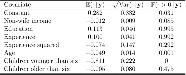
We also report the model parameter estimates for the probit model for τ = 10 in Table 2, together with the posterior standard deviations and the probabilities that the parameters are positive. All parameter estimates have signs that are consistent with economic theory. For instance, non-wife income, age and the number of children in the household have a negative impact on the probability that an average woman will participate in the labor market. On the other hand, education and experience both have a positive impact, though the impact of experience is diminishing (the impact is quadratic in years of experience). However, note the large posterior standard errors for the coefficients associated with the variables experience squared and children older than six.

Table 2: Parameter posterior means, standard deviations, and probabilities being positive for the probit model.

Covariate E(_{· |}y) pVar(_{· |}y) P(_·>0_|y) Constant 0.282 0.832 0.631 Non-wife income ₋0.012 0.009 0.085 Education 0.113 0.046 0.995 Experience 0.100 0.041 0.992 Experience squared ₋0.074 0.147 0.292 Age ₋0.049 0.014 0.001 Children younger than six ₋0.811 0.222 0 Children older than six ₋0.005 0.080 0.475

5.1.3 Comparison with Other Methods

and Chib and Jeliazkov (2001) (for Metropolis-Hastings output), and we refer to this the CJ method. We use each of the three methods to estimate the marginal likelihoods of the three binary response models, and compare the methods in terms of computation time and numerical accuracy. Implementation details are given as follows. For the CE method, we first useL= 2500 MCMC draws to compute the optimal importance sampling density for each of the three models, and then sampleN = 50000 draws from the density obtained for the main importance sampling run. For both the GD-G and CJ methods, we use L = 50000 MCMC draws to estimate the marginal likelihood. But instead of one long chain, we run 10 parallel chains each of length

L= 5000, so that the numerical standard errors of the estimates can be readily computed.2

It is worth noting the different factors affecting the computation times of the three methods. Since both the GD-G and CJ methods require a lot of MCMC draws, when those draws are more costly to obtain (e.g., more costly in the t-link model than in the probit model), both methods tend to be slower. When reduced runs are required, as in the logit model, the CJ method tends to be slower (the other two methods do not require reduced runs). Finally, when the evaluation of the (integrated) likelihood function is more costly (e.g., more costly in the

t-link model than in the probit model), the GD-G and CE methods — both require numerous evaluations of the likelihood function — tend to be slower.

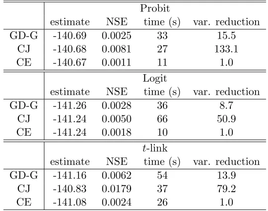
Table 3: Log marginal likelihood estimate, numerical standard error, and computation time (in second) for the three methods. Variance reduction is approximately the amount of time needed to have the same level of accuracy as the CE method.

Probit

estimate NSE time (s) var. reduction GD-G -140.69 0.0025 33 15.5

CJ -140.68 0.0081 27 133.1 CE -140.67 0.0011 11 1.0

Logit

estimate NSE time (s) var. reduction GD-G -141.26 0.0028 36 8.7

CJ -141.24 0.0050 66 50.9 CE -141.24 0.0018 10 1.0

t-link

estimate NSE time (s) var. reduction GD-G -141.16 0.0062 54 13.9

CJ -140.83 0.0179 37 79.2 CE -141.08 0.0024 26 1.0

We report in Table 3 the marginal likelihood estimate (in log), its numerical standard error and the computation time (in second) for each of the three methods. For all the binary response models, the proposed CE method is both the quickest and provides the most accurate estimates. To compare the methods with the same denominator, we also provide the “variance reduction” of the CE method compared to the other two methods. For example, to achieve the same level of accuracy as the CE method for estimating the marginal likelihood of the probit model, the

2

More precisely, the numerical standard error is calculated as the sample standard deviation of the 10 estimates divided by√

GD-G method would take about 15.5 (33/11 _×(0.0025/0.0011)2) times longer than the CE method. It is obvious from the results that the CE method provides substantial improvements over the other two competing methods.

5.2 Vector Autoregressive Models for U.S. Macroeconomic Time Series

In the second empirical application we analyze a dataset obtained from the US Federal Reserve Bank at St. Louis website3

that consists of 248 quarterly observations from 1948Q1 to the 2009Q4 on n= 4 U.S. macroeconomic series: output (GDP) growth, interest rate, unemploy-ment rate, and inflation.

One fundamental question is: which time-series specification considered previously in the litera-ture best models the evolution and interdependence among the time series? To make a first step towards answering this question, we perform a formal Bayesian model comparison exercise to compare three popular time-series specifications. The first model we consider is a basic vector autoregressive (VAR) model. Pioneered by Sims (1980), it has traditionally been employed to capture the interdependence among the time series. Specifically, for t = 1, . . . , T, we consider the first-order VAR model

yt=µ+Γyt−1+εt, εt∼N(0,Ω), (12)

where yt is a vector containing measurements on the aforementioned n = 4 macroeconomic

variables (output growth, unemployment, income, and inflation),µis an n_×1 vector of inter-cepts, Γ is an n_×n matrix of parameters that governs the interdependence among the time series, and Ω is an unknown n_×n positive definite covariance matrix. The analysis is per-formed conditionally on the initial data point and consequently our sample consists ofT = 247 observations.

For the purpose of estimation, (12) is rewritten in the form of a seemingly unrelated regression (SUR) model as follows:

yt=Xtβ+εt, (13)

whereXt=I⊗(1,y′t−1),βis aq×1 (q =n 2

+n) vector containing the corresponding parameters from µ and Γ, ordered equation by equation, i.e., β = vec ((µ,Γ)′_{), and the vec(·) operator} stacks the columns of a matrix into a vector. Stacking the observations in (13) over t, we have

y=Xβ+ε, ε_∼N_(0,I⊗Ω),

where

y=

  

y1

.. .

yT

 

, X=

  

X1

.. .

XT

 

, ε=

  

ε1

.. .

εT

  .

Although the traditional VAR model is a popular specification for macroeconomic series, it is not flexible enough to accommodate potential structural instabilities in the times series. In view of this, in our second specification we extend the basic VAR model (12) by allowing the parameter vectorβ to evolve over time in order to study the potential structural change of the time series.

3

In particular, we consider the following first-order time-varying parameter vector autoregressive (TVP-VAR) model (e.g., Canova, 1992; Carter and Kohn, 1994; Koop and Korobilis, 2010):

yt=µt+Γtyt−1+εt, εt∼N(0,Ω), (14)

where the parametersµ_tandΓtnow have a subscripttto denote the time period. The evolution

of the parameter vectorβ_t= vec ((µ_t,Γt)′) fort= 2, . . . , T is governed by the evolution equation

β_t=β_t−1+νt, (15)

withβ1∼N(0,D), whereνt∼N(0,Σ), andΣ= diag(σ21, . . . , σ2q) is an unknownq×qdiagonal

matrix. The transition equation (15) allows the elements of β_t to evolve gradually over time by penalizing large changes between successive values, thus a priori favoring the simple VAR model with time-invariant parameters.

Another approach to extend the traditional VAR model (12) is the following dynamic factor VAR (DF-VAR) model (e.g., Bernanke et al., 2005; Koop and Korobilis, 2010):

yt=µ+Γyt−1+Aft+εt, εt∼N(0,Ω), (16)

whereΩ= diag(ω2 1, . . . , ω

2

n) is a diagonal matrix,Ais ann×1 vector of factor loadings, andft

is an unobserved factor that captures economy-wide macroeconomic volatility, which is assumed to evolve as

ft=γft−1+ηt, ηt∼N(0, σ

2

f), (17)

fort= 2, . . . , T, and the initial factor f1 is distributed according to the stationary distribution

f1 _∼ N_{(0, σ}2

f/(1 −γ

2

)) with _|γ_| < 1. Since neither the factor loadings A nor the factorft is

observed, the scale and sign ofAandftare not individually identified becauseAft= (cA)(ft/c)

for anyc₆= 0. One popular identification assumption is to fixed the first element ofA at 1, i.e.,

A= (1,a′)′ and ais an (n₋1)_×1 vector of free parameters. With this assumption, both the sign and scale identification problems are resolved.

5.2.1 The Priors and Marginal Likelihood Estimation

In this subsection we describe the priors used in the three models and provide the implementa-tion details of the proposed importance sampling approach. Since the value of marginal likeli-hood in general is sensitive to the choice of priors, we maintain the same priors across models where appropriate. In addition, we consider a set of reasonable yet relatively non-informative priors in a prior sensitivity analysis to see how the marginal likelihood estimates are affected by the choice of priors.

For the VAR model, the parameters are β and Ω with independent prior distributions: Ω_∼ IW_{(ν0,S0) and β ∼} N_{(β0,Vβ), where} IW_{(·,·) is the inverse-Wishart distribution, ν0 = n+} 3,β0 =0 and Vβ = 10×I. These are conjugate priors and are standard in the literature. For

S0 we consider two cases: S0=IandS0 = 0.1×I. Standard results from the SUR model can be

applied to sample from the posterior density, e.g., see Koop (2003). To estimate the marginal likelihood of the model, we consider the parametric family_F =_{fN(β;b,B)fIW(Ω;ν,S)_}, where

fIW(_·;ν,S) is the density of IW_{(ν,S). Given the posterior output {βl,Ωl}}L

reference parameters bband Bb can be obtained as in (11). As for bν and Sb, first note that

b

S−1 = 1

νL

L

X

l=1 Ω−_l 1.

Now by substituting S = Sb−1 into the density fIW(_·;ν,S), ν_b can be obtained by any one-dimensional root-finding algorithm (e.g., Newton-Raphson method). Alternatively, simply fixing

b

ν =T also gives reasonable results. The former approach is the one we use for the empirical example.

For the TVP-VAR model, we assume that Ω _∼ IW_{(ν0,S0) and each diagonal element of Σ} follows, independently, an inverse-gamma distribution: σ2

i ∼ IG(ν0i/2, S0i/2), for i = 1, . . . , q,

with D= 10_×I,ν0 =n+ 3, and ν0i = 6, S0i = 0.01 fori= 1, . . . , q. For S0, we consider two

cases: S0 =I and S0 = 0.1×I. Posterior inference is based on a recently proposed algorithm

in Chan and Jeliazkov (2009), which we briefly describe in the appendix. More importantly for our purpose, Chan and Jeliazkov (2009) also give an efficient way to evaluate the integrated likelihood, defined as the likelihood function marginal of the state vectorβ. Hence, to compute the marginal likelihood of the TVP-VAR model, we can work with the integrated likelihood

f(y_|Ω,Σ) rather than the complete-data likelihoodf(y_|β,Ω,Σ). This approach substantially reduces the variance of the importance sampling estimator as we analytically “integrate out”

β that consists of 247 β_t’s, each of which is a 20-dimensional vector. Generally, in situations where the integrated likelihood f(y_|θ) cannot be efficiently evaluated, one has to work with the complete-data likelihood f(y_|z,θ), where z is the latent variable vector. The proposed approach proceeds as before, with the optimal importance densityf(θ,z;bvce) constructed from

the posterior draws. In this case, however, the variance of the associated estimator is no smaller than the case where integrated likelihood f(y_|θ) can be efficiently evaluated. Now, to obtain the optimal importance density for the TVP-VAR model, we consider the parametric family

F =_{fIW(Ω;ν,S)

q

Y

i=1

fIG(σ2_i;mi, si)}.

The optimal CE parameters _{ν,_b Sb_} are obtained as in the previous case. Moreover, since the inverse-gamma density is a special case of the inverse-Wishart density, (m_bi,bsi), i= 1, . . . , q can

be obtained similarly.

Lastly, the priors for the parameters in the DF-VAR model are given as follows: β_∼N_(β0,Vβ), a_∼N_{(a0,Va), andγ is distributed uniformly on the interval (−1,1), withβ0 =0,Vβ = 10×I} and a0 = 0. For Va, we consider two cases Va = I and Va = 5 ×I. In addition, each

diagonal element ofΩ= diag(ω2 1, . . . , ω

2

q) follows, independently, an inverse-gamma distribution:

ω2

i ∼ IG(ν0i/2, S0i/2), for i = 1, . . . , q, and finally, σ2 ∼ IG(νf, Sf), where νf = ν0i = 6,

Sf = S0i = 1. Posterior inference is based on an efficient MCMC sampler discussed in Chan

and Jeliazkov (2009). Specifically, instead of sequentially drawing from the full conditionals, we implement the following collapsed Markov sampler that substantially improves the mixing properties and reduces the autocorrelation of the Markov chain:

Algorithm 3. Collapsed MCMC Sampling of β and A

1. [β_|y,A,Ω, γ, σ2

2. [a,f_|y,β,Ω, γ, σ2], which is done using

(a) [a_|y,β,Ω, γ, σ2

], which does not depend onf (b) [f_|y,β,A,Ω, γ, σ2

]

3. [Ω_|y,β,A,f]

4. [γ_|f, σ2

]

5. [σ2

|f, γ]

Now, to locate the optimal importance density, we consider the following parametric family

F =

(

fN(θ;bθ,Bθ)fN(γ;bγ, Bγ)fIG(σ

2

;m, s)_}

q

Y

i=1

fIG(ω_i2;mi, si)

)

,

where θ = (β′,a′)′_{. Since the densities are either normal or inverse-gamma, the optimal CE} reference parameters can be obtained exactly in the same way as before.

5.2.2 Empirical Results

1960 1980 2000 −1

−0.5 0 0.5

GDP growth equation

1960 1980 2000 −0.4

−0.2 0 0.2 0.4 0.6

Inflation rate equation

1960 1980 2000 −0.5

0 0.5 1 1.5

Unemployment equation

1960 1980 2000 −1

0 1 2 3

Interest rate equation

µ_t−1 GDP

t−1 inflationt−1 unempt−1 interestt−1

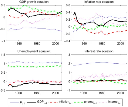
Figure 1: Evolution of the parameters β_t in the TVP-VAR model.

1950 1960 1970 1980 1990 2000 2010 ft

−4 −3 −2 −1 0 1 2 3

Figure 2: Evolution of the latent dynamic factor ft in the DF-VAR model, together with the

timing of officially announced U.S. recessions (shaded regions).

To formally compare the three time-series specifications, we compute the marginal likelihoods for the models via the proposed importance sampling approach. More specifically, for each model, we first use the posterior draws to estimate the optimal CE reference parameters for the importance density. Then we obtain an estimate for the marginal likelihood via importance sampling (which involves only normal and inverse-Wishart distributions) with a sample size of

N = 10000. In particular, no reduced MCMC runs nor auxiliary simulations are needed. More-over, should the researcher desire a more accurate estimate, additional draws can be obtained from the importance density with little computational costs. A prior sensitivity analysis is also done following the procedure described in Section 4. More particularly, for each model only one Markov sampler is run, and the MCMC draws are used to estimate the marginal likelihoods un-der both prior specifications. The estimated log marginal likelihoods are verified by the method of Chib and Jeliazkov (2001). The estimates, together with the numerical standard errors, are reported in Table 4. The result suggests that the TVP-VAR model is the best model for the U.S. post-war data among the three, under a variety of prior specifications. However, the relative ranking of the VAR and DF-VAR models changes as we use different priors, highlighting the importance of a prior sensitivity analysis in marginal likelihood estimation.

Table 4: Log marginal likelihood (numerical standard error) for the three time-series models.

VAR TVP-VAR DF-VAR

S0 =I S0= 0.1×I S0 =I S0 = 0.1×I Va= 5×I Va=I

−905.4(0.005) ₋925.6(0.005) ₋899.8(0.24) ₋896.0(0.61) ₋906.0(0.46) ₋903.9(0.28)

5.2.3 Comparison with Other Methods

Geweke (1999) (GD-G method) and the method of Chib (1995) and Chib and Jeliazkov (2001) (CJ method). We use each of the three methods to estimate the marginal likelihoods of the three VAR models, and compare the methods in terms of computation time and numerical accuracy.

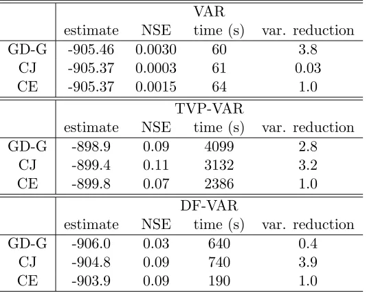
Table 5: Log marginal likelihood estimate, numerical standard error, and computation time (in second) for the three methods. Variance reduction is approximately the amount of time needed to have the same level of accuracy as the CE method.

VAR

estimate NSE time (s) var. reduction GD-G -905.46 0.0030 60 3.8

CJ -905.37 0.0003 61 0.03 CE -905.37 0.0015 64 1.0

TVP-VAR

estimate NSE time (s) var. reduction GD-G -898.9 0.09 4099 2.8

CJ -899.4 0.11 3132 3.2 CE -899.8 0.07 2386 1.0

DF-VAR

estimate NSE time (s) var. reduction GD-G -906.0 0.03 640 0.4

CJ -904.8 0.09 740 3.9 CE -903.9 0.09 190 1.0

First, for computing the marginal likelihood of the VAR model via the CE method, we use

L = 2500 MCMC draws to obtain the optimal importance sampling density, and then sample

N = 100000 draws from the density obtained for the main importance sampling run. For both the GD-G and CJ methods, we useL= 50000 MCMC draws to estimate the marginal likelihood. Again, instead of one long chain, we run 10 parallel chains each of length L= 5000, such that the numerical standard error of the estimate can be computed easily. We report in Table 5 the estimate (in log), its numerical standard error and the computation time (in second) for each of the three methods, as well as the approximate amount of time needed to have the same level of accuracy as the CE method. For this relatively low-dimensional model, all three methods work very well, and the CJ method gives the most accurate estimate per unit of computation time.

We then perform the same exercise for the TVP-VAR model. The CE method uses L= 5000 MCMC draws for obtaining the optimal importance sampling density andN = 100000 draws for the main importance sampling run; both the GD-G and CJ methods use L= 100000 MCMC draws. Estimation of the marginal likelihood is much more time-consuming for this high-dimensional model: the GD-G, CJ and CE methods take respectively 68, 52 and 40 minutes. For the TVP-VAR model, the CE method is the fastest and most accurate. For instance, the CJ method would need about 129 minutes to achieve the same level of accuracy as the CE method (which takes only 40 minutes).

draws. Although the CE method is the fastest, the GD-G method seems to provide the most accurate estimate given the same computation time. However, it is also worth noting that the GD-G estimate is slightly different from those obtained via the CJ and CE methods (taking into account of the small numerical standard errors), and this might indicate that the bias of the GD-G estimate in this example is substantial.

6

Concluding Remarks

In this article we introduce the CE method to tackle an important problem in Bayesian econo-metrics and statistics, namely, the estimation of marginal likelihood. Although the problem is well-studied and many approaches already exist, the proposed method has the merit of being both conceptually and computationally simple. In particular, it is essentially an importance sampling approach, with the choice of importance density guided by a methodology founded on formal optimization by minimizing the cross-entropy distance to the posterior density (i.e. the intractable zero-variance importance density). Therefore, the importance density is cho-sen to systematically minimize the variance of the resulting estimate, yet random samples can be obtained from it conveniently with negligible computational costs. Furthermore, since the draws are independent by construction, the simulation effort is much less compared to other approaches should one wish to reduce the numerical standard error of the estimator. In the two empirical applications studied, the CE method compares favorably to existing estimators.

Generally, this approach relies on the researcher designating afamily of densities on which the CE-based optimization method is implemented to operate. For many applications, as demon-strated through two empirical examples in the text, this choice of distribution family is relatively straightforward. Typically, it will be sufficient to match the chosen family with the class of prior distributions employed by the model. Regardless of the family chosen, however, the eventual optimization over this collection, as prescribed by the CE approach, amounts to an exercise directly analogous to likelihood maximization.

This suggests, therefore, that when a particular choice of distribution family is inadequate, straightforward extensions are readily available. For example, it may be worthwhile to consider expanding a family of multivariate normal distributions to one consisting of amixture of mul-tivariate normal distributions. Such a generalization presents little additional computational difficulties – multivariate normal mixture likelihoods, while no longer analytically tractable, are easily maximized by Expectation-Maximization based techniques. To that end, an interesting and important extension of the algorithm presented in this paper would be one incorporating the automatic selection of the parametric family. We leave the latter open for future work.

Appendix A: Efficient Simulation of the Gaussian State Space

Models

In this appendix we present an efficient Markov sampler proposed in Chan and Jeliazkov (2009) for simulation and integrated likelihood estimation in state space models. We consider the following linear Gaussian state space model:

yt = Xtβ+Gtηt+εt, (18)

η_t = Ztγ+Ftηt−1+νt, (19)

fort= 1, . . . , T, whereytis ann×1 vector of observations,ηtis aq×1 latent state vector, (19)

is initialized withη1∼N(Z1γ,D), and

εt νt ∼N 0,

Ω11 0 0 Ω22

.

Equation (18) is often referred to as the measurement or observation equation, while (19) is called the transition or evolution equation. Definey= (y1, . . . ,yT) andη= (η1, . . . ,ηT), and

let θ represent the parameters in the state space model (i.e. β,γ,_{Gt},{Ft}, and the unique

elements of Ω11, Ω22, andD). The covariates {Xt} and {Zt} are taken as given and will be

suppressed in the conditioning sets below.

From (18)–(19) it is easily seen that the joint sampling densityf(y_|θ,η) is Gaussian. In fact, stacking (18)–(19) over theT time periods, we have

y=Xβ+Gη+ε,

where X=    X1 .. . XT  

, G=

   G1 . .. GT  

, ε=

   ε1 .. . εT   ,

withε_∼N_{(0,I⊗Ω11). A change of variable from εto y implies that}

f(y_|θ,η) =fN(y_|Xβ+Gη,I_⊗Ω11). (20)

For the prior distribution ofη, we note that the directed conditional structure forf(η_t|θ,η_t−1)

in (19) implies that the joint density forη is also Gaussian. To see this, define

H=        I

−F2 I

−F3 I

. .. ... −FT I

      

and S=

       D Ω22 Ω22 . .. Ω22        ,

so that (19) can be written as Hη=Zγ+ν, where

Z=    Z1 .. . ZT  

 and ν =

   ν1 .. . νT  

Therefore, by a simple change of variable from ν to η, we have

η_|θ_∼N _ηe,K−1_{, (21)}

whereηe=H−1Zγ and theT q_×T q precision matrixK is given byK=H′S−1H, i.e.,

K=

      

F′2Ω− 1

22F2+D−1 −F′2Ω− 1 22

−Ω−221F2 F′3Ω

−1

22F3+Ω− 1

22 −F′3Ω

−1 22

. .. . .. . ..

−Ω−221FT−1 F′_TΩ22−1FT +S−221 −F′_TΩ− 1 22

−Ω−221FT Ω−221

      

.

(22) It is important to realize that the precision matrix K is block-banded and contains a small number of non-zero elements in a narrow band around the main diagonal. This observation is important as it affords substantial saving in storage space and computation costs.

Since the densities f(y_|θ,η) and f(η_|θ) in (18) and (19) are both Gaussian, the standard update for Gaussian linear regression (see, e.g. Koop, 2003; Gelman et al., 2003) implies that the conditional posterior densityf(η_|y,θ)_∝f(y_|η,θ)f(η_|θ) is also Gaussian:

η_|y,θ _∼N_(ηb,P−1_{), (23)}

where the precision Pand the mean bη are given by

P = K+G′ I_⊗Ω−111

G, (24)

b

η = P−1 Kη_e+G′ I_⊗Ω−111

(y₋Xβ). (25)

Since G′ I_⊗Ω−111

Gis banded, it follows thatP is also banded. This allows samplingη_|y,θ

without the need to carry out an inversion to obtain P−1 and bη in (25). Specifically, the mean

b

ηcan be found in two steps. First, we compute the (banded) Cholesky factor CofPsuch that

C′C=P. Second, we solve

C′Cηb=Kηe+G′(I_⊗Ω−111)(y−Xβ), (26)

forCη_bby forward-substitution and then using the result to solve forbηby back-substitution. The two steps are done in_O(T q2

) operations. Similarly, to obtain a random draw from N_(ηb,P−1₎ efficiently, sample u _∼ N_{(0,I), and solve Cx = u for x by back-substitution. It follows that} x_∼ N_(0,P−1

). Adding the mean ηb to x, one obtains a draw η _∼N_(ηb,P−1

). We summarize the above procedures in the following algorithm.

Algorithm 4. Efficient State Smoothing and Simulation

1. Compute P in (24) and obtain its Cholesky factor Csuch that P=C′C.

2. Smoothing: Solve (26) by forward- and back-substitution to obtain _bη.

3. Simulation: Sample u_∼N_{(0,I), and solveCx=u for x by back-substitution and take}

Lastly, we describe an efficient method to evaluate the integrated likelihoodf(y_|θ), defined as

f(y_|θ) =

Z

f(y_|θ,η)f(η_|θ)dη, (27)

wheref(y_|θ,η) is the likelihood andf(η_|θ) represents the prior. This quantity is often used in likelihood evaluation for classical and Bayesian problems involving optimization and model comparison. Evaluating the integrated likelihood via the multivariate integration in (27) is computationally intensive and often impractical. However, the derivation of the full condi-tional density f(η_|y,θ) discussed above provides a simple way to evaluate f(y_|θ) without invoking (27). Specifically, it follows from the Bayes’ theorem that integrated likelihood as

f(y_|θ) = f(y|θ,η)f(η|θ)

f(η_|y,θ) , (28)

where f(η_|y,θ) denotes the full conditional posterior density of η given (y,θ). Due to the banded nature of the prior and posterior precision matrices (KandP, respectively), evaluation of the integrated likelihoodf(y_|θ) at the pointθcan be done efficiently simply by evaluating the right-hand-side of (28) at a single point (θ,η). Note that the choice is arbitrary, in particular, the choice η =ηb eliminates the need to compute the exponential part of the density function in the denominator density.

Appendix B: Proofs of Propositions

Proof of Proposition 1. We prove the claims for the VM estimator; the proof for the CE esti-mator follows similarly. We first show that the marginal likelihood p(y) is finite for any given

y. Using Assumption 1 and the fact that the prior is proper, we have

p(y) =

Z

p(y_|θ)p(θ)dθ 6p(y_|bθ)

Z

p(θ)dθ =p(y_|bθ)<_∞.

Now write the VM estimator as the the average of N iid copies of the random variableZn:

b

pvm(y) = 1

N

N

X

n=1 Zn,

whereZn=p(y|θn)p(θn)/f(θn;v∗vm) and θn∼f(θn;v∗vm). It is easy to see that

EZn=

Z

p(y_|θn)p(θn)

f(θn;v∗vm)

f(θn;v∗vm)dθn=

Z

p(y_|θn)p(θn)dθn=p(y)<∞.

Therefore, by the (weak) law of large number, pvm_b (y) converges in probability to p(y) as

N _{→ ∞}. Next, note that

E[_bpvm(y)] =E

"

1

N

N

X

n=1 Zn

#

= 1

N

N

X

n=1

p(y) =p(y). (29)