Derivative of a Determinant with Respect to an Eigenvalue
in the LDU Decomposition of a Non-Symmetric Matrix
Mitsuhiro Kashiwagi
Department of Architecture, School of Industrial Engineering, Tokai University, Toroku, Kumamoto, Japan Email: mkashi@ktmail.tokai-u.jp
Received October 11, 2012; revised November 11, 2012; accepted November 18, 2012
ABSTRACT
We demonstrate that, when computing the LDU decomposition (a typical example of a direct solution method), it is possible to obtain the derivative of a determinant with respect to an eigenvalue of a non-symmetric matrix. Our pro- posed method augments an LDU decomposition program with an additional routine to obtain a program for easily evaluating the derivative of a determinant with respect to an eigenvalue. The proposed method follows simply from the process of solving simultaneous linear equations and is particularly effective for band matrices, for which memory re- quirements are significantly reduced compared to those for dense matrices. We discuss the theory underlying our pro- posed method and present detailed algorithms for implementing it.
Keywords: Derivative of Determinant; Non-Symmetric Matrix; Eigenvalue; Band Matrix; LDU Decomposition
1. Introduction
In previous work, the author used the trace theorem and the inverse matrix formula for the coefficient matrix ap- pearing in the conjugate gradient method to propose a method for derivative a determinant in an eigenvalue problem with respect to an eigenvalue [1]. In particular, we applied this method to eigenvalue analysis and dem- onstrated its effectiveness in that setting [2-4]. However, the technique proposed in those studies was intended for use with iterative methods such as the conjugate gradient method and was not applicable to direct solution methods such as the lower-diagonal-upper (LDU) decomposition, a typical example. Here, we discuss the derivative of a determinant with respect to eigenvalues for problems in- volving LDU decomposition, taking as a reference the equations associated with the conjugate gradient method [1]. Moreover, in the Newton-Raphson method, the solu- tion depends on the derivative of a determinant, so the result of our proposed computational algorithm may be used to determine the step size in that method. Indeed, the step size may be set automatically, allowing a reduc- tion in the number of basic parameters, which has a sig- nificant impact on nonlinear analysis. For both dense ma- trices and band matrices, which require significantly less memory than dense matrices, our method performs cal- culations using only the matrix elements within a certain band of the matrix factors arising from the LDU decom- position. This ensures that calculations on dense matrices proceed just as if they were band matrices. Indeed,
computations on dense matrices using our method are expected to require only slightly more computation time than computations on band matrices performed without our proposed method. In what follows, we discuss the theory of our proposed method and present detailed algo- rithms for implementing it.
2. Derivative of a Determinant with Respect
to an Eigenvalue Using the LDU
Decomposition
The eigenvalue problem may be expressed as follows. If A is a non-symmetric matrix of dimension n n , then the usual eigenvalue problem is
Ax x, (1) where and x denote respectively an eigenvalue and an corresponding eigenvector. In order for Equation (1) to have nontrivial solutions, the matrix AI must be singular, i.e.,
detAI0. (2) We introduce the notationf
for the left-hand side of this equation:
detf AI. (3) Applying the trace theorem, we obtain
1
1
trace
trace
f
A I A I
f
A I
where
11
21 22
1 2
ij
n n nn
a
a a
A I a
a a a
. (5)
The LDU decomposition decomposes this matrix into a product of three factors:
ALDU, (6) where the L, D, and U factors have the forms
21 1 2 1 1 1 ij n n L
, (7)
11 22 ij nn d d D d d
, (8)
12 1 2 1 1 1 n n ij u u u U u
. (9)
We write the inverse of the L factor in the form
21 1 1 2 1 1 1 ij n n g L g g g
. (10)
Expanding the relation (where I is the iden- tity matrix), we obtain the following expressions for the elements of :
1 LL I
1 L
1 ij ij
i j g ,
1
1
2
i
ij ij ik kj
k j
i j g g
. (11)Next, we write the inverse of the U factor in the form
12 1 2 1 1 1 1 n n ij h h h U h
. (12)
Expanding the relation , we again obtain expressions for the elements of :
1
U U I
1
U
1 ij ij
j i h u , 1
1
2
j
ij ij kj ik
k i
j i h u u h
. (13)Equations (11) and (13) indicate that gij and ij
must be computed for all matrix elements. However, for matrix elements outside the half-band, we have ij
h
0
and uij 0, and thus the computation requires only ele- ments ij and uij within the half-band. Moreover, the
narrower the half-band, the more the computation time is reduced.
From Equation (4), we see that evaluating the deriva- tive of a determinant requires only the diagonal elements of the inverse of the matrix A in (6). Using Equations (7)- (10), and (12) to evaluate and sum the diagonal elements of the product U D L1 1 1, we obtain the following rep- resentation of Equation (4):
1 11
n n
ki ik
i ii k i kk
f g h
f d
d . (14)This equation demonstrates that the derivative of a de- terminant may be computed from the elements of the inverses of the , , and matrices obtained from the LDU decomposition of the original matrix. As noted above, the calculation uses only the elements of the ma- trices within a certain band near the diagonal, so compu- tations on dense matrices may be handled just as if they were band matrices. Thus we expect an insignificant in- crease in computation time as compared to that required for band matrices without our proposed method.
L D U
By augmenting an LDU decomposition program with an additional routine (which simply appends two vectors), we easily obtain a program for evaluating f f . Such computations are useful for numerical analysis using algorithms such as the Newton-Raphson method or the Durand-Kerner method. Moreover, the proposed method follows easily from the process of solving simultaneous linear equations.
3. Algorithms for Implementing the
Proposed Method
3.1. Algorithm for Dense Matrices
We first discuss an algorithm for dense matrices. The arrays and variables are as follows.
1) LDU decomposition and calculation of the deriva- tive of a determinant with respect to an eigenvalue
(1) Input data
A: given coefficient matrix,
2-dimensional array of the form A(n,n)
b: work vector, 1-dimensional array of the form b(n) c: work vector, 1-dimensional array of the form c(n) n: given order of matrix A and vector b
eps: parameter to check singularity of the matrix (2) Output data
ierr; error code
=0, for normal execution =1, for singularity
(3) LDU decomposition do i=1,n
<d(i,i)> do k=1,i-1
A(i,i)=A(i,i)-A(i,j)*A(j,j)*A(j,i) end do
if (abs(A(i,i))<eps) then ierr=1
return end if
<l(i,j) and u(i,j)> do j=i+1,n do k=1,i-1
A(j,i)=A(j,i)-A(j,k)*A(k,k)*A(k,i) A(i,j)=A(i,j)-A(i,k)*A(k,k)*A(k,j) end do
A(j,i)=A(j,i)/A(i,i) A(i,j)=A(i,j)/A(i,i) end do
end do ierr=0
(4) Derivative of a determinant with respect to an ei-genvalue
fd=0 <(i,i)>.
do i=1,n
fd=fd-1/A(i,i) end do
<(i,j)> do i=1,n-1 do j=i+1,n b(j)=-A(j,i)
c(j)=-A(i,j) do k=1,j-i-1
b(j)=b(j)-A(j,i+k)*b(i+k) c(j)=c(j)-A(i+k,j)*c(i+k) end do
fd=fd-b(j)*c(j)/A(j,j) end do
end do
2) Calculation of the solution (1) Input data
A: L matrix, D matrix and U matrix, 2-dimensional array of the form A(n,n) b: given right-hand side vector,
1-dimensional array of the form b(n) n: given order of matrix A and vector b (2) Output data
b: work and solution vector, 1-dimensional array (3) Forward substitution
do i=1,n
do j=i+1,n
b(j)=b(j)-A(j,i)*b(i) end do
end do
(4) Backward substitution do i=1,n
b(i)=b(i)/A(i,i) end do
do i=1,n ii=n-i+1 do j=1,ii-1
b(j)=b(j)-A(j,ii)*b(ii) end do
end do
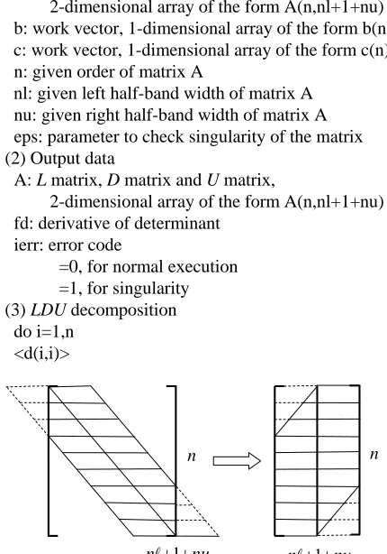
3.2. Algorithm for Band Matrices
We next discuss an algorithm for band matrices. Figure 1 depicts a schematic representation of a band matrix. Here denotes the left half-bandwidth, and de- notes the right half-bandwidth. These numbers do not include the diagonal element, so the total bandwidth is
n
1
n n
nu
u
.
1) LDU decomposition and calculation of the deriva- tive of a determinant with respect to an eigenvalue
(1) Input data
A: given coefficient band matrix,
2-dimensional array of the form A(n,nl+1+nu) b: work vector, 1-dimensional array of the form b(n)
c: work vector, 1-dimensional array of the form c(n) n: given order of matrix A
nl: given left half-band width of matrix A nu: given right half-band width of matrix A eps: parameter to check singularity of the matrix
(2) Output data
A: L matrix, D matrix and U matrix,
2-dimensional array of the form A(n,nl+1+nu) fd: derivative of determinant
ierr: error code
=0, for normal execution =1, for singularity
(3) LDU decomposition do i=1,n
<d(i,i)>
n
nu
[image:3.595.315.530.406.713.2]n1 n1nu n
do j=max(1,i-min(nl,nu)),i-1 A(i,nl+1)=A(i,nl+1)
-A(i,nl+1-(i-j))*A(j,nl+1)*A(j,nl+1+(i-j)) end do
if (abs(A(i,nl+1))<eps) then ierr=1
return end if
<l(i,j)>
do j=i+1,min(i+nl,n) sl=A(j,nl+1-(j-i)) do k=max(1,j-nl),i-1 sl=sl-
A(j,nl+1-(j-k))*A(k,nl+1)*A(k,nl+1+(i-k)) end do
A(j,nl+1-(j-i))=sl/A(i,nl+1) end do
<u(i,j)>
do j=i+1,min(i+nu,n) su=A(i,nl+1+(j-i)) do k=max(1,j-nu),i-1
su=su-A(i,nl+1-(i-k))*A(k,nl+1)*A(k,nl+1+(j-k)) end do
A(i,nl+1+(j-i))=su/A(i,nl+1) end do
end do ierr=0
(4) Derivative of a determinant with respect to an ei-genvalue
fd=0 <(i,i)>
do i=1,n
fd=fd-1/A(i,nq) end do
<(i,j)> do i=1,n-1
do j=i+1,min(i+nl,n) b(j)=-a(j,nl+1-(j-i)) do k=1,j-i-1
b(j)=b(j)-a(j,nl+1-(j-i)+k)*b(i+k) end do
end do do j=i+nl+1,n b(j)=0.d0 do k=1,nl
b(j)=b(j)-a(j,k)*b(j-nl-1+k) end do
end do
do j=i+1,min(i+nu,n) c(j)=-a(i,nl+1+(j-i)) do k=1,j-i-1
c(j)=c(j)-a(i+k,nl+1+(j-i)-k)*c(i+k) end do
end do
do j=i+nu+1,n c(j)=0.d0 do k=1,nu
c(j)=c(j)-a(i,nl+1+k)*c(j-nl-1+k) end do
end do do j=i+1,n
fd=fd-b(j)*c(j)/a(j,nl+1) end do
2) Calculation of the solution (1) Input data
A: given decomposed coefficient band matrix, 2-dimensional array of the form A(n,nl+1+nu) b: given right-hand side vector,
1-dimensional array of the form b(n) n: given order of matrix A and vector b
nl: given left half-band width of matrix A nu: given right half-band width of matrix A
(2) Output data
b: solution vector, 1-dimensional array (3) Forward substitution
do i=1,n
do j=max(1,i-nl),i-1
b(i)=b(i)-A(i,n+1-(i-j))*b(j) end do
end do
(4) Backward substitution do i=1,n
ii=n-i+1
b(ii)=b(ii)/a(ii,nl+1) do j=ii+1,min(n,ii+nu)
b(ii)=b(ii)-a(ii,nl+1+(j-ii))*b(j) end do
end do
4. Conclusion
determinant with respect to an eigenvalue. The result of this computation is useful for numerical analysis using such algorithms as those of the Newton-Raphson method and the Durand-Kerner method. Moreover, the proposed method follows easily from the process of solving simul- taneous linear equations and should prove an effective technique for eigenvalue problems and nonlinear prob- lems.
REFERENCES
[1] M. Kashiwagi, “An Eigensolution Method for Solving the Largest or Smallest Eigenpair by the Conjugate Gradient Method,” Transactions of the Japan Society for Aeronau- tical and Space Sciences, Vol. 1, 1999, pp. 1-5.
[2] M. Kashiwagi, “A Method for Determining Intermediate Eigensolution of Sparse and Symmetric Matrices by the Double Shifted Inverse Power Method,” Transactions of JSIAM, Vol. 19, No. 3, 2009, pp. 23-38.
[3] M. Kashiwagi, “A Method for Determining Eigensolu- tions of Large, Sparse, Symmetric Matrices by the Pre- conditioned Conjugate Gradient Method in the General- ized Eigenvalue Problem,” Journal of Structural Engi- neering, Vol. 73, No. 629, 2008, pp. 1209-1217. [4] M. Kashiwagi, “A Method for Determining Intermediate
Eigenpairs of Sparse Symmetric Matrices by Lanczos and Shifted Inverse Power Method in Generalized Eigenvalue Problems,” Journal of Structural and Construction Engi- neering, Vol. 76, No. 664, 2011, pp. 1181-1188.