Munich Personal RePEc Archive
Income Heterogeneity and
Environmental Kuznets Curve in Africa
Ogundipe, Adeyemi and Alege, Philip and Ogundipe,
Oluwatomisin
Covenant University, Ota
3 May 2014
1 INCOME HETEROGENEITY AND ENVIRONMENTAL KUZNETS CURVE IN AFRICA
Adeyemi A. Ogundipea
Philip O. Alegea (Ph.D)
Oluwatomisin M. Ogundipea
a
Department of Economics and Development Studies, Covenant University, Ota, Ogun State, Nigeria
Corresponding email: ade.ogundipe@covenantuniversity.edu.ng +2348161927372
Abstract
The Environmental Kuznets Curve (EKC) hypothesis asserts that pollution levels rises as a country develops, but reaches a certain threshold where pollution begins to fall with increasing income. In EKC analysis, the relationship between environmental degradation and income is usually expressed as a quadratic function with turning point occurring at a maximum pollution level. The study seeks to examine the pattern and nature of EKC in Africa and major income groups according to World Bank classification comprising low income, lower middle income and upper middle income in Africa. In ensuring the robustness of our study; the paper proceeded by ascertaining the nature of EKC in all fifty-three countries of Africa in order to confirm the results obtained from basic and augmented EKC model. The study could not validate EKC hypothesis in Africa (combined), low income and upper middle income but empirical and analytical evidences supports the existence of EKC in lower middle income countries. Likewise, evidences from the robustness checks confirmed the findings from the basic and augmented EKC model. The study could not attain a reasonable turning point as there are evidences that Africa could be turning on the EKC at lower levels of income. Also, there is need to strengthen institutions in order to enforce policies that prohibits environmental pollution and ensure pro-poor development.
Keywords: Pollution, Income, Environmental Kuznets Curve, Africa
JEL Classification: Q5, O4, Q1, N17
2 1.0 Introduction
The concept of EKC originates from Kuznets (1955) who hypothesized that income inequality
first rises and then falls as economic development proceeds but the concept actually emerged via
the path breaking study of Grossman and Krueger on the potential environmental impacts of
NAFTA in 1991. The Environmental Kuznets Curve (EKC) hypothesized the relationship
between per capita income and indicators of environmental degradation. It suggests that in the
early stages of economic growth degradation and pollution increases but beyond some level of
income per capita which will vary for different indicators, the trend reverses, so that high income
levels leads to environmental improvement. It hereby implies that the environmental impact
indicator is an inverted U-shaped function of income per capita (Stern 2009). According to
Lomborg (2001) who draws on the World Bank’s World Development Report (1992) which
contained one of the first environmental Kuznets curve (EKC) studies, later published by Shafik
(1994). The EKC refers to an empirical finding which indicates an inverted U-Shaped
relationship between local air pollution and per capita income.
An attempt to validate EKC model has results into diverse results in Africa, with empirical
studies of Baliamoune-Lutz (2012); Osabuohien, Efobi and Gitau (2014) validating the
hypothesis while Omotor and Orubu (2001); Orubu and Awopegba (2009) failed to confirm the
existence of EKC. The mixed findings arising from the empirical investigation of EKC could
have arisen from income heterogeneity in Africa economies. Since income and development
levels differ among these economies, the realization (non-realization) of EKC in Africa cannot
be used to affirm the existence (non-existence) of EKC in individual Africa economies. Perman
and Stern (2003) argued that there is a doubt on the general applicability of EKC because even
when cointegration relationship was established between variables in regions, many of the
relationships for individual countries were not concave. Therefore, this present re-examination of
EKC model in Africa controls for cross country income heterogeneity by grouping Africa
economies based on World Bank classifications of low income, lower middle income and upper
middle income and investigated the nature of EKC in each income group accordingly. More so,
in validating the result from our model and extant studies, this current attempt ascertained the
3 The hope for the future is conditional on decisive political action now to begin managing
environmental resources to secure both sustainable human progress and human survival. Inquest
for every nation to actualize some economic successes, there has been obvious threat to the
environment. Each year witnesses several hectares of productive dry-land turns into worthless
desert, likewise more than 11 million hectares of forests are destroyed yearly. In Europe, acid
precipitation kills forests and lakes and damages the artistic and architectural heritage of nations.
The world is experiencing global warning arising from consistent burning of fossil fuels into the
atmosphere. The green house effect has the potential to mitigate agricultural production, raise sea
levels to flood coastal cities and disrupt national economies (UN Environmental Report 1993).
Other industrial gases threaten to deplete the planet’s protective ozone shield to such an extent
that the number of human and animal cancers would rise sharply and the oceans’ food chain
would be disrupted. From the foregoing and the popularization of EKC, it becomes clear that the
acquisition of economic growth and the need to ensure cleaner quality environment are
inseparable issues. Many forms of development erode the environmental resources and on the
long-run environmental degradation can jeopardize economic development. In an attempt to
ensure realization of present needs that will not distort the ability of the future generations to
meet their needs; there is need for policy makers, national government and international
institutions to implement policy and guidelines for production and extractive processes and
enforce adequate abatement measures (Alege and Ogundipe 2013).
Our work is related to numerous attempts to explain the pollution growth nexus. Most studies
test the validity of the so called EKC hypothesis which postulates an inverted U-shaped
relationship between environmental degradation and income growth (see Grossman and Krueger
1994 and 1995)
The study conducts inferences on the relationship between the development stage and pollution
dynamics of Africa countries in order to draw policy implications. Our study emphasize a
dynamic processes where the relationship between environmental degradation and income levels
is considered, disaggregating Africa economics into low income, lower middle income, upper
middle income and high income countries. Though, erstwhile study on the subject matter
(Osabuohien et al., 2014) have aggregated the economies of Africa but considering the intent of
4 income; it becomes imperative to disaggregate countries according to income level. Our study
hereby attempt to ascertain if a country’s income level does matter for its pollution dynamics;
since its current development stage influences its future pollution prospect. Also, examine the
pattern and direction of relationship between pollution and income; and determine the speed of
realization of EKC (if it does exist) in the face of various interventions/abatement measures. This
enables policy makers and environmental activist to ensure appropriate actions needed to assume
sustainable development.
The remaining part of the paper is structured as follows: section two situates the experience of
Africa with the rest of the world and analyses the CO2 emissions and income relationships in
income groups in Africa; section three outlines the related literature that situate our study in the
context of existing literature; section four put forward the model appropriate for empirically
investigation of EKC in Africa; sections five discusses the empirical results and findings from
our estimation procedure while section six concludes the paper and offers policy
recommendations.
2.0 Stylized Facts/Background Information
This section presents the state of environmental pollution in Africa in comparison to the rest of
the world. Figure one shows that CO2 emission has consistently maintain an upward trend in
Africa and the rest of the world. This form the reason for the establishment of Kyoto protocol
and initialization of commitment to reduce the level of CO2 emission since it constitute the
largest contributor to the share of total green house gases (GHGs) in the world (Bank Bank,
2007). In the same manner, table one shows the regional contribution to world CO2 emissions,
with Africa share steadily increasing raging from 1.78 percent to 2.5 percent and eventually 2.17
percent in period 1971-1980, 1981-1990 and 2001-2010 respectively. In relative terms, Africa
has contributed minimally to the world CO2 emissions when compared to other regions. East
Asia and pacific contributes 15.56 percent, 25.55 percent and 30.84 percent in the same periods.
Likewise Europe, Latin America and Middle East have contributed more than 5 percent (between
5 and 30 percent) to CO2 emissions for the observed periods. In spite of Africa lower relative
contributions; Osabuohien et al (2014) claimed that in absolute terms, CO2 is has risen
5
Figure1: Trend of CO2 emissions (kt) and GDP Per Capita in Africa
Authors’ computation from WDI (2013)
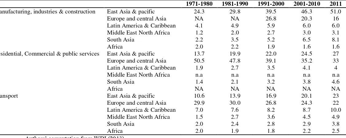
Also, table 2 shows the sectoral contributions to world CO2 emissions according to six regional
divisions for which statistics were available. As seen in the table 2, East Asia and pacific
accounts for the largest CO2 emissions in manufacturing, industries and construction sectors with
about 60 percent rise in the period 1970-2011. Likewise, Europe, Latin America and Middle East
share witnessed steadily increase while Africa’s contribution dwindles overtime. This evidence would not be unconnected to the weak manufacturing capacity and industrial exports in Africa,
which contributes less than 10 percent to merchandise exports. More so, due to high fossil fuel
consumption in Africa; the transport sector share of world emissions has maintain an upward
trend from 2 percent in 1971-1980 to about 3 percent in 2011. Likewise, the same upward trend
was witnessed in Latin America, Middle East and South Asia while Europe and central Asia
reduce the level of transport CO2 emissions. This is likely due to adoption of clean technologies
as a result of increased income levels and development.
0
200000
400000
600000
800000
C
O
2
1960 1970 1980 1990 2000 2010 year
CO2 emission in Africa
600
700
800
900
1000
P
C
I
1960 1970 1980 1990 2000 2010 year
6
Table 1: CO2 emissions (kt) as a percentage contribution to the world CO2 emissions
Regions 1971-1980 1981-1990 1991-2000 2001-2008
East Asia & Pacific 15.65 19.52 25.55 30.84
Europe & Central Asia n.a n.a 29.71 23.77
Latin America & Caribbean 4.00 4.66 5.16 5.18
Middle East North Africa 2.94 3.88 5.20 6.09
South Asia 1.75 2.90 4.59 5.58
Africaa 1.78 2.27 2.15 2.17
Authors’ computation from WDI (2013)
Note: n.a means not available
a Sub-Saharan is used to capture Africa, as Africa was not classified in the WDI data base
Following the assertion from Grossman and Krueger (1991); the pollution-income relation
relationship income tends to rise with increasing income at early growth stages. However,
reaching a threshold (turning point) environment begins to improve at higher stages of growth.
This assertion is reflected in the so called inverted U-shaped curve, expressing the relationship
between pollution and income. As seen in figure 2, we could not ascertain the direction of
pollution-income relationship until the point USD800; from this point, the pattern became stable
and consistent with expected behavior at early growth stages but yet to witnessed an identifiable
turning point. If the empirical claim of Omotor and Orubu (2012) is to be relied upon, the curve
might experience a threshold at about USD1344.63, from which higher level of growth will lead
to improving the environment.
Figure 2: Pattern of Pollution-income relationship in Africa
Authors’ computation from WDI (2013)
C
O
2
700 800 900 1000
PCI
[image:7.612.71.366.459.673.2]7 The major threat towards environment centres on how to ensure sustainable environment, adopt
cleaner environment and adopt abatement measures in the face of poverty in the developing
economies. Poverty is adjudge a major cause of environmental problems in developing
economies; balancing the immediate needs of survival with long run sustainability is the issue at
hand and requires policy interventions capable of reducing extreme poverty and extent of income
inequality. The foregoing are the concerns that lead to the establishment of the world
[image:8.612.31.595.240.466.2]commission on environment and development by UN General Assembly in 1993.
Table 2: Sectoral CO2 emission as percentage contribution to the World sectoral CO2 emissions
1971-1980 1981-1990 1991-2000 2001-2010 2011
Manufacturing, industries & construction East Asia & pacific 24.3 29.8 39.5 46.3 51.0
Europe and central Asia NA NA 26.8 20.3 16
Latin America & Caribbean 4.1 4.9 5.9 6.0 6.0
Middle East North Africa 1.2 2.0 2.7 3.0 3.1
South Asia 2.2 3.5 5.2 6.5 8.1
Africa 2.0 2.2 1.9 1.6 1.6
Residential, Commercial & public services East Asia & pacific 13.7 19.9 22.0 24.5 27
Europe and central Asia 50.5 47.8 39.1 35.2 33
Latin America & Caribbean 1.9 2.7 3.5 4.1 4
Middle East North Africa n.a n.a n.a n.a n.a
South Asia 1.4 2.1 3.2 3.8 4.6
Africa NA NA NA NA NA
Transport East Asia & pacific 10.6 13.9 16.9 20.1 23
Europe and central Asia 29.9 30.0 26.8 24.3 22
Latin America & Caribbean 7.0 7.6 8.2 8.7 10.0
Middle East North Africa 1.5 2.7 3.6 4.5 4.9
South Asia 2.0 2.4 2.8 2.9 3.8
Africa 2.0 1.9 1.8 2.2 2.5
8
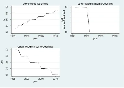
Figure 3: Group CO2 emissions (kt) as percentage contribution to Africa’s CO2 emissions
Authors’ computation from WDI (2013)
It becomes clear from evidences in figure 3 and table 3, that poverty fuels environmental
degradation in Africa. The carbon dioxide CO2 share of the low income countries (which
constitute 51 percent of Africa economies) in Africa’s total of CO2 emissions has been raising
steadily, from 53 percent in 1996 to 60 percent in 2011. Whereas, the share of GDP Per Capita of
these economies in Africa’s’ average has fallen considerably over the same period. This singular
fact that have accounted for mixed finding on the nature of EKC in Africa, since extant failed to
control of income differences across Africa economies. This, as well confirms the words of
Lipfert (2004) that “though poor people may be more susceptible, but poverty also fosters
increased pollution”. In the spirit of EKC, Hollander (2003) describes the problem of poor as unable to deal with pollution until they acquire affluence to meet their basic needs for survival.
Table 3: GDP Per Capita & CO2emission as percentage contribution to Africa’s total
Year/group
1996 2000 2006 2011
PCI CO2 PCI CO2 PCI CO2 PCI CO2
Low income 29.3 53.5 24.0 55.2 21.2 57.3 22.2 59.3
Lower middle income 92.2 22.3 84.0 22.6 84.4 22.0 89.4 21.6
Upper middle income 363 22.9 374 21.7 345 20.2 313 18.6
Authors’ computation from World Development Indicators (WDI) (2013)
52 54 56 58 60 LI
1995 2000 2005 2010 year
Low Income Countries
22 2 2 .2 2 2 .4 2 2 .6 2 2 .8 23 L M I
1995 2000 2005 2010 year
Lower Middle Income Countres
19 20 21 22 23 U M I
1995 2000 2005 2010 year
[image:9.612.69.466.634.707.2]9 A critical observation of table 3 shows that statistics available in different income groups does
not validate the EKC hypothesis except in the lower middle income group. In low income Africa,
CO2 emissions rises as per capita income falls; CO2 rises from 53.5 percent in 1996 to 57.3
percent and 59.3 percent in 2006 and 2011 respectively. Also, in the upper middle income group,
the share of GDP Per Capita in Africa’s average falls consistently with CO2 emissions indicating
a U-shaped relationship. Contrarily, in the lower middle income, emissions falls from 22.6
percent in 2000 to 22 percent in 2006 and further to 21.6 percent in 2011 while GDP Per Capita
share rises from 84 percent to 84.8 percent and peak at 89.4 percent in 2000, 2006 and 2011
respectively. The trend witnessed in the lower middle income group validates the inverted
U-shaped hypothesis of EKC.
The evidence in table 3 re-affirm the core thrust of this study and the need to control for income
heterogeneity in ascertaining the pattern and nature of EKC in Africa and as well examines the
specific nature and turning points in individual country.
3.0 Review of Related Literature
The EKC theme was popularized by the World Bank’s world development Report 1992 (IBRD
1992) which argued that: “the view that greater economic activity inevitably hurts the
environment is based on static assumptions about technology, tastes and environmental
investments” and that “as income rise, the demand for improvements in environmental quality will increase, as will the resources available for investment. Other have also expounded this
position even more forcefully, for instance Beckerman (1992) claimed that “there is clear
evidence that, although economic growth usually leads to environmental degradation in the early
stages of the process, in the end the best and probably the only way to attain a decent
environment in most countries is to become rich”.
According to Cole 2003; Lomborg (2001) in his book skeptical environmentalist shared the
opinion of Beckerman (1992) strongly. Lomborg argues that although air pollution emissions are
rising in many developing countries, the EKC indicates that it is possible to “grow out” of
environmental problems through technological advance and environmental policy. Thus, he
claims that today’s developing countries should one day experience the reductions in pollutions
10 pollutants have fallen steadily in the developed world over the last 30-40 years. Lomborg (2001)
confirmed this assertion by providing emissions and concentrations trends for the UK and the
USA and the USA for lead, particulates, sulphur dioxide, nitrogen dioxide, and carbon monoxide
and concludes that air quality in these countries has significantly improved.
Asserting from the study conducted by Grossman and Krueger (1995); Cole et al (1993); Alege
and Ogundipe (2013); the EKC relationship is typically explained in terms of the interaction of
scale, composition and technique effects. The scale effect indicates that, ceteris paribus,
economic growth will increase pollution1. However, with increasing per capita income, the
economy experiences a compositional change from manufacturing to services; the effect of these
changes would likely result in reducing pollution intensity of output. More so, as the nation
continue to experience a leap in per capita income and as welfare improves, it is argued that the
demand for cleaner environment rises culminating into positive income elasticity of demand for
environmental quality and ultimately increase demand for environmental regulations. In the
words of Cole 2003; this resultant changes to the technique of production are known as the
technique effect. The combination of technique and composition effects therefore eventually
outweighs the scale effect, resulting in the downturn of EKC.
Considering the composition effect; there seem to be a challenge for LDCs (most especially
resource-abundant LDCs). The case of LDCs may not follow the same pollution income path
experienced in developed economies. If the pollution intensity of output has fallen in the North
as a result of the Migration of heavy industry to the South due to i. proximity to resource area ii.
proximity to market iii. Market displacement of Northern industries by Southern industries iv.
Strict environmental regulation in the North etc; then, it is unlikely that the south can expect to
enjoy similar reductions in pollution intensity. The study by Suri and Chapman (1998) found
lower emissions with increased manufactured imports and found higher emissions with increased
exports; it hereby suggests that compositional changes, as reflected in changing trade patterns,
are influencing energy consumption and hence pollution.
Likewise, there are inherent problem in developing countries that could mitigate the transition
from scale to composition effect; this factors include i. attraction of dirty industries into the
1
11 extractive industry ii. weak governance and heavy incidence of corruption iii. weak
environmental regulation and lack of enforcement, and iv. extremely skewed income, which
continually widen inequality gap and subjected the poor to degrading the environment to
maintain survival. Cole (2000) also find that the increasing cleanliness of the composition of
manufacturing sector is at least partly responsible for falling pollution in the developed world.
Contrarily, Janicke et al., (1997) shows that the North is still a net exporter of many pollution
intensive products, suggesting that each compositional changes may not be as significant as
proposed. Though, pollution haven hypothesis2 has found limited support (mani and wheeler
1998; Lucas et al., 1992; Birdsaff and wheeler 1993) likewise some empirical studies documents
a little evidence of the formation of pollution havens (Xu and Song 2000; Tobey 1990; Van
Beers and Van De Bergh 1997). Contrarily, the work of Antweiler et al (2001); Cole and Elliot
(2003) found evidence of pollution haven pressures. This is likely to have resulted from the fact
that many pollution intensive sectors in the LDCs are highly capital intensive and most suited for
the capital abundant North.
Also, it is generally recognized that environmental concern is income elastic; countries and
social groups increase their interest in environmental quality as their income rise (Ruttan 1971;
Ciriacy-wantrup 1963; Chapman and Barker 1991). If environmental improvement is to succeed
increased income, there seems to be a problem for Africa, especially the natural resources
dependent economies. The rent-seeking behavior of multinationals and economic agents
involved extraction which arises from weak institutions tends to dissipate the benefits of
economic resources and lengthen the vicious cycle of poverty. Since, most rural poor depends on
local economic activities for survival; as the level of poverty expands, environmental
degradation worsens. Crudely put by Chapman 1993; at population-intensive subsistence levels,
rural households are more interested in consuming wildlife than its protection for the
enhancement of future generation. As the economy grows; there is need for policies that will
enhance both natural living standard and environmental protection in the world’s poorest
countries.
Perrings (1989, 1991), clark (1991), and Ciricay-wantrup (1963) have argued that low income
causes high discount rates. If this is correct, it confirms the widely shared observation that very
2
12 poor regions seem to degrade renewable resources stocks far below economically optimal levels
(Chapman 1990, Moyo 1991).
Grossman and Krueger (1991) in their pioneer study of EKC investigating the potential
environmental impacts of NAFTA. They developed a cross-country panel that estimated EKCs
for SO2, dark matter (fine smoke), and Suspended particles (SPM) using global environmental
Monitoring system (GEMS) data set for 42 developing and developed countries3. The empirical
work by Grossman and Krueger found evidence supporting EKC patterns for SO2 and SPM; the
turning point for both pollutants are precisely estimated at $4772-5965 while the concentration
of suspended particles appeared to decline even at low income levels. Following the idea of
Grossman and Krueger (1991), Shafik and Bandhopadhyay (1992) were first to conduct a major
empirical study in ascertaining the EKC hypothesis. The study adopted different functional
relationship to estimate EKCs for ten indicators; EKC was not attained for deforestation.
However, lack of clean water and lack of urban sanitation were found to decline uniformly with
increasing income over time. Contrarily, municipal waste and carbon emissions per capita
increased unambiguously with rising income, while river quality tended to worsen with
increasing income.
Naimzada and Sodini (2010) examine the dynamics of an OLG model with environment, a CES
production function and agents who invest in environment, taking the action of other agents of
the same generation as given. The authors show the possibility of a high income, low
environment steady-state when total factor productivity increase over a threshold value and the
elasticity of substitution between capital and labour is sufficiently lower. Varvarigos (2010)
studies a model where: (a) longevity is positively affected by public health spending and
negatively influenced (b) environmental degradation is positively influenced by pollution due to
production and it is mitigated by public environment expenditure. He proves that low income –
low pollution equilibra are possible depending on the elasticity of (i) environmental damage with
regard to pollution (ii) environmental improvements with respect to abatement policy. The
likelihood of traps is also a function of the cleanliness of production technology, total energy
prodcutivity and initial conditions.
3
13 Our work is related to numerous attempts to explain the pollution growth nexus. Most studies
test the validity of the so called Environmental Kuznets Curve hypothesis, which postulates an
inverted U-shape relationship between environmental degradation and income (Grossman and
Krueger, 1994 and 1995; Osabuohien et al., 2014; Beckerman 1992; Stern 2003); while others
such as (Agra and Chapman 2008; Galeotti et al., 2006; Coondoo and Dinda 2008) failed to
validate the hypothesis. Although numerous studies test the EKC hypothesis, for individual
countries (friedl and Getzner 2003; Roca et al., 2001; De Bruyn et al 1998; Roberts and Grimes
1997) and panel of countries (canes et al 2003; stern 2004; Perman and Stern 2003; Huang and
Cin 2007) empirics have failed to yield conclusive result (Aslanidis 2009; Soyas and Sari 2009;
Bassetti et al.,). Moreover, most empirical studies are considered to be econometrically weak
(Stern 2004; Narayan and Narayan, 2010; Brock and Taylor, 2010). In a recent study, Narayan
and Narayan 2010 examine the EKC hypothesis in a panel of 43 developing countries using
panel cointegration in order to overcome econometric pitfalls. They conclude that CO2
emissions fall as income rises only in Middle Eastern and South Asian countries. Finally, Brock
and Taylor (2010) employ the Green Solow model as an alternative framework and present
robust evidence of convergence between the 173 countries examined using standard panel
technique.
In a parallel strand of research, environmental convergence (using CO2 emissions) is examined.
In recent work, Bulte et al., (2007) argue that income convergence leads to pollutant emissions
convergence. Overall findings on environmental convergence alone are contradictory, as a
number of scholars support the hypothesis of convergence in CO2 emissions per capita
(Strazicish and Lit 2003; Romero-Avila 2008; Westerland and Basher 2008) whereas others
provide evidence of divergence (Nguyen-Van 2005; Barassi et al., 2008). Finally, in a study
related to our work, Aldy (2006) shows that markov chain analysis does not provide convincing
evidence on future emissions convergence. The author finds evidence of convergence among 23
OECD countries, whereas emissions appear to be diverging for a global sample composed 88
countries for 1960-2000. Xepapadeas (1997) analyses an endogenous growth model with
productive and abatement capital as well as increasing returns due to knowledge spillovers in
production and pollution abatement. He shows that countries with environmental concerns can
be trapped in a low growth, high pollution equilibrium because of insufficient knowledge of
14 4.0 Methodology
The study adopted a standard presentation and framework of basic EKC model as presented in
Chapman and Agra (1999); Omotor and Orubu (2003); Al sayed and Sek (2013).
According to Wen and Cao (2009), the theoretical interpretation of the sign and relationship of the parameters4 is below:
a. indicate linear shape and monotonically increasing. As income rises, environmental pressure is increasing
b. represent linear shape and monotonically decreasing. As income rises, environmental pressure is decreasing
c. indicate U-shape; as reaches a threshold, environmental pressure decreases as income rises
d. indicate U-shape
e. indicate N-shape, similar to U-shape. But as income rises further, environmental pressure increases again
f. indicate reserve N-shape, environmental pressure decreases first; then increases and later decreases
g. indicate horizontal line, income does not affect environmental pressure
Presenting our simple EKC model in a panel framework, we have
Where represents environmental degradation,
is GDP per capita, and
represents the slope of the model, and are the intercept parameter; represents the
cross-section of countries or regions and denotes the years or periods of time series and . Hence,
the implicit assumption is that, although environmental degradation/quality may be different
between one country and the other at any given level of income. The income elasticity is the
same for all countries at given level of income. On the other hand, the time specific intercepts
4
15 take care of time-varying variables that are omitted from the model, including stochastic shocks
(Omotor and Orubu, 2001).
In order to establish the stability of EKC model, we introduce other variables relevant in
explaining the extent of environmental degradation. According to Chapman and Agras (1999),
all empirical investigations of EKC adopts a functional forms capable of evaluating results with
respect to the presence or absence of a turning point and the significance of its parameters. The
analysis of the relationship of the effect of real per capita income on environmental degradation
controlling for other variables relevant to the argument usually assume the form presented
below:
Where is a vector of explanatory variables added to the basic EKC model; such that
Here, represents population density (people per sq. km of land area), is external
debt stock, is an indicator manufactured exports, is human capital, is
environmental official development assistance, and is a measure of institutions (regulatory
quality). The turning point value is
The specification above is similar to the stand by Khanna (2002); who suggested income as one
of the factors necessary to ascertain exposure to declining environmental quality; other factors
such as race, education, population density, housing tenure and structural composition of
workforce are also relevant (Panayotou 1997; Torres and Boyce 1998). In the words of Omotor
et al., (2012) finding an EKC in the presence of other modifying factors provides a more
persuasive basis for validating the hypothesis. In the model above, the basic EKC model was
augmented to include factors such as population density, external debt stock, manufactured
exports, and regulatory quality. The higher the population density, the greater will be the
intensity of pollution and pressure on environmental services and resources. The inclusion of
16 (1994); Suri and Chapman (1998). If the sign of turns negative, it implies high
emissions with increased export, otherwise export mitigate the level of emission.
4.1 Technique of Estimation
We adopted the panel data analysis to detect the nature of the EKC curve between the pollutants
and the economic growth. Panel data helps to determine dynamic of changes in short time series
and provides more powerful regression by considering the place (spatial) and time (temporal)
dimensions of the data (Schmidheiny and Basel, 2011). It as well helps to control for
unobservable individual heterogeneity across entities. There are two types of panel model
namely; the fixed effect (FE) model and the random effect (RE) model.
The fixed effect model is used in analyzing the impact of variables that vary overtime; it explores
the relationship between predictor and outcome variables within an entity5. The fixed effect
removes the effect of those time invariant characteristics from the predictor variables in order to
assess the predictors’ net effect. The equation for the fixed effect model is shown as:
Where is the unknown intercept for each entity (n entity specific intercepts),
is the dependent variable where = entity and = time, represents the vector of independent
variable, are time invariant or fixed over time and captures the error term. The structure of
the model to be estimated with the fixed effected is stated as follows
Where
is the unknown intercept for each country.
According to Alege and Ogundipe (2014); the fixed model is relevant as it enables us to sieve
5
17 out the unobserved effect across entities, hereby making changes in dependent variable to be
absolutely explained by influences from the observed pollution predictors.
The random effect model, unlike the fixed, it assumes that variations across countries are random
and uncorrelated with the independent variables. The random effect specification takes the mean
error and random term as randomized. Both error components are assumed to be random
variable with normal distribution which is identically independent distributed ( ). these error
components are uncorrelated with independent variable (Yaffee 2013; Al sayed and Sek 2013;
Alege and Ogundipe 2014), such that:
In choosing the consistent and efficient model between the fixed effect and random effect model;
we adopted the Hausman test. The test is considered as a Wald test with ( degrees of
freedom where is the number of regressors in the model. The Hausman statistic is model as
follow:
Where
Under random effects model, the matrix difference in brackets is positive, as the random effects
estimator is efficient and any other estimator has a larger variance. Under the null hypothesis,
both FE and RE model are consistent with RE more consistent. Under the alternative hypothesis,
FE is more efficient than RE. Therefore, the rejection of null hypothesis will suggest the choice
of FE model (Yaffee, 2003; Al Sayed and Sek, 2013).
4.2 Data Sources and Measurement
The data series required to empirically investigate the nature of EKC in Africa and the major
income classification groups were sourced from the World development indicators of the World
Bank 2013. These variables include; environment degradation proxied with Carbon dioxide
(CO2) emissions, gross domestic per capita income, population density, stock of external debt
while manufactured export and regulatory quality were obtained from the data market of Iceland
18
Table 4: Data Sources and Measurement
Variable Symbol Sources measurement
Environmental degradation GDP Per Capita
Evdg gpci
World Development Indicators (WDI) World Development Indicators (WDI)
CO2 emissions in Kilowatt tons
Constant $US
Population density Pden World Development Indicators (WDI) People per Sq. km of land area
External debt Extd World Development Indicators (WDI) Total external debt stock
Manufactured export Mfxp Data market of Iceland Constant $US
Regulatory quality Regq World Governance Indicators (WGI) Units
5.0 Discussion of Result
In an attempt to ascertain the pattern and nature of EKC in Africa, the study begins by estimating
the basic EKC model for Africa and various income groups according to the World Bank
classifications. The models were estimated using both fixed and random effects and the hausman
test was conducted to determine a reliable and consistent model. The fixed effect result was
found consistent for Africa and Upper middle income model while the random effect result was
consistent for Low income and Lower middle income models.
The result readily available in the table below could not ascertain the existence of EKC in Africa,
low income and upper middle income economies. Also, there exist an inverse relationship
between economic degradation (CO2 emissions) and income (GDP Per Capita) at the early stage
of development. This reflects the extent of income inequality and the fact that the growth effort
of most Africa economies is not geared toward the poor. Following the decision criteria of EKC
parameter, especially from quadratic GDP Per Capita; the empirical investigation from Africa,
Low income economies and Upper middle income economies shows evidence in support of a
U-shaped relationship between pollution and income. Contrarily, the study confirms the EKC
hypothesis in lower middle income countries though no reasonable turning point could be
ascertained. The realization of EKC in lower middle income countries and the positive
relationship between CO2 emissions and income at the early development stage is hinged on the
reality that about 70 percent of economies in this category are oil exporting countries. Since gas
flaring constitute a major source of CO2 among Africa oil producing economies and oil proceeds
in most cases account for over 90 percent foreign earnings; there tends to exist a natural
relationship between emissions and environmental degradation in Lower middle income
19
Table 5: Basic EKC model for Africa
Variable Africaa Low incomeb Lower middlec Upper middled
Lpci -0.4217 -2.1578* 4.5566* -6.2293
lpci2 0.1311* 0.2871* -0.2189** 0.4608
C 4.5422* 9.7915* -13.2790* 28.5235
F-test Prob.* 0.0000 0.0000
W-test Prob.* 0.0000 0.0000
Hausman 14.47* 3.57 0.04 8.39*
EKC No No Yes No
Obs 758 435 192 116
Authors’ computation using Stata 11.0
Note: a Africa is the EKC result for fifty three Africa countries b Low income comprises thirty countries with GDP Per Capita of $1,035 or less c Lower middle comprises fourteen countries with GDP Per Capita between $1,036 to $4085 d Upper middle comprises of eight countries with GDP Per Capita between $4,086 to $12, 615
The study proceeds to estimate the expanded EKC model for Africa and the income groups. A
similar estimation procedure was conducted, this include the pooled ordinary least square, the
fixed effect and random effect model. The fixed effect results satisfied the requirement of
efficiency and consistency as shown by the hausman test for all groups except the upper middle
income Africa where random effect appears to be more efficient. Though the result presented in
table 6 is an augmentation of the basic EKC model; the nature and pattern of EKC remain as
obtained in the basic model. The empirical results from our study was consistent with Omotor
and Orubu and Orubu (2012) who failed to achieve EKC for lack of access to safe water using 24
Africa countries. Also our evidences match the studies of Galeotti et al., (2006) and Coondoo
and Dinda (2008) who could not find evidence to affirm the validity of EKC hypothesis for
non-OECD countries; but inconsistent with Orubu and Awopegba (2009) and Osabuohien et al.,
(2014) who established EKC for CO2 emissions in Africa. More so, as shown in the augmented
EKC analysis, population density exerts a significant positive influence on environmental
degradation. It implies that as population density intensifies, more pressure is exerted on
economic resources and environmental services; most especially in the quest for livelihood. This
is a major experience in most Africa’s semi urban and rural communities where major means of livelihood is agriculture; activities ranging from local mining, deforestation, bush burning, etc.
have contributed to eroding environmental quality.
Also, the indicator of external debt (asides from Africa as a whole) was found statistically
significant for only low income group, since almost all the economies in this category are heavily
20 for financing debt service and repayment tends to create more pollution and environmental
degradation. Finally, the measure of institution (regulatory quality) was found significant across
groups except in lower middle income, where EKC was realized. There is the need to strengthen
regulatory quality in other income groups to adherence to environmental regulations, adoption of
21
Table 6: Expanded EKC model for Africa
Variable Africa Low income Africa Lower middle income Africa Upper middle income Africa
Pols Fixed Random Pols Fixed Random Pols Fixed Random Pols Fixed Random
lpci -0.7208 1.5327** 1.5628* 2.3417 2.6891* 2.5382** 34.3933* 1.2465 4.6914 -9.5786** -7.6913 -9.578**
lpci2 0.0983** -0.0395 -0.0409 -0.1272 -0.1296 -0.1145 -2.2426* -0.0302* -0.2635 0.5611* 0.4725*** 0.5611**
lpden 0.1355** 0.4884** 0.3460* 0.1344** 0.4513* 0.1765** 1.7141* 0.9192** 0.7109** 1.9654* 1.2424* 1.9654*
lextd 0.9431** 0.0502** 0.0754** 0.6377* 0.0804* 0.1166* 1.5003* 0.0473 0.1453** -0.0371 -0.0344 -0.0371
lmxp 0.1165** 0.0131 0.0409* 0.1839* -0.0377 0.1141 -0.0478 0.0708 0.1158* -0.0295 -0.0376 -0.0295
re 0.0212 -0.1084** -0.1101** -0.2952* -0.0894** -0.1023* -1.8143* -0.1549 -0.1643 -0.1680* -1.5834** -0.1680*
c -14.888 -3.1766 -4.0435** -19.6984* -6.4194** -6.6966*** -162.9025* -4.7539 -20.1052*** 48.3631* 40.6901** 48.3631*
F-(prob.*) 0.0000 0.0000 0.0000 0.0000 0.0000 0.0000 0.0000 0.0000
R2 0.7395 0.7263 0.8240 0.9990
W-(prob.*) 0.0000 0.0000 0.0000 0.0000
Hausman YES
14.47*
YES 12.84*
YES 19.28*
YES 2.53* Pesaran
test
1.155 (0.2479)
1.5372 (0.351)
1.8266 (0.352)
-1.321 (0.427)
Wald test 5702.80 200.45 11390.9
LM test 1.63
(0.2011) Authors’ computation using stata 11.0
Note: Pols indicates ordinary pooled regression estimates
In ensuring the reliability of our estimates for policy inferences, decision making and forecasting; the study conducted some
sensitivity checks which include:
i. The Pesaran cross sectional dependence/contemporaneous correlation test. This is imputed as simply pesaran test in table 6. The
pesaran test was conducted to test whether the residuals are correlated across entities; it becomes expedient to verify as cross
sectional dependence can lead to a bias in test results. With the probability value of 0.2479, the study accepted the null hypothesis
22 ii. The Modified Wald test for groupwise heteroskedasticity in fixed effect regression model,
here the study failed to reject the null hypothesis of homoskedasticity or constant variance.
This implies that our model is homoskedastic and hereby appropriate.
iii. Brensch-Pagan Lagrange multiplier (LM) test for random effects. The LM test helps to
decide between a random effect regression and a simple OLS regression. The null hypothesis
in the LM test suggests that variance across entities is zero, that is, no significant difference
across units. Here, the study failed to reject the null; therefore, random effect is not
[image:23.612.63.556.270.615.2]appropriate or does not significantly differ from pooled OLS.
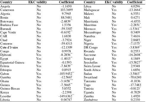
Table 7: EKC Model for Africa Economies
Country EKC validity Coefficient Country EKC validity Coefficient
Angola No -1.1650 Libya No 4.0296
Cameroon No 103.3699 Madagascar Yes -13.1664**
Algeria No 9.7965 Malawi No 6.5551
Benin No 88.5481 Mali No 0.4271
Botswana Yes -2.6839** Mauritania No -4.6553
Burkina Faso No 1.5356 Mauritius Yes -2.2851*
Burundi No -59.3307 Morocco Yes -1.5341**
Cape Verde Yes -0.6192** Mozambique No 0.3409
CAR No 1.6830 Namibia No 7.4616
Chad No -3.7924 Niger No 2.8685
Comoros No -59.4313 Nigeria Yes -7.1375*
Cote d’lvoire No -12.1309 DR Congo Yes -3.8369**
Congo No 0.9978 Rwanda No 0.2553
Djibouti Yes -8.2856** Sao tome Yes -16.2608**
Egypt Yes -1.4013** Senegal No 4.1849
Equatorial Guinea No -0.1593 Seychelles Yes -15.5827**
Eritrea Yes -7.8439** Sierra Leone No 2.9348
Ethiopia No 0.8915 South Africa No 1.6856
Gabon Yes -105.9452** Sudan Yes -3.5843**
Gambia No -12.5667 Swaziland No -70.6240
Ghana Yes -3.1458*** Tanzania Yes -0.1036
Guinea Yes -7.5665** Togo No -17.7483
Guinea-Bissau No 5.8552 Tunisia Yes -0.8123*
Kenya No -2.2398 Uganda No -0.7029
Lesotho Yes -149.6362** Zambia No 1.4920
Liberia No 0.04747 Zimbabwe No 0.2330
Authors’ computation using stata 11.0
The study also examine the pattern of EKC in individual countries of Africa, this is conducted to
ensure the robustness of our parameter estimates and results. The results obtained confirm the
foregoing analytical and empirical stands reached in previous sections. The estimation process
23 Also, out of the nineteen that supported EKC hypothesis, ten were from the lower middle income
group. Following the facts obtained from our analytical and empirical analyses, it therefore
becomes imperative for policy makers to tread with caution on the implementation of findings
and recommendation from erstwhile studies.
6.0 Conclusion and Recommendation
The study examines the pattern and nature of EKC in Africa and major income groups according
to the World Bank income classification comprising low income, lower middle income and
upper middle income in Africa. Also, for the purpose of ensuring robustness, the study
ascertained the pattern of EKC in all Africa countries. We adopted a panel estimation procedure
based on ordinary pooled regression, fixed and random effect regression and attained an efficient
and consistent model with the aid of hausman model selection test. More so, for the purpose of
ensuring reliability of our parameter estimation for policy inferences, we carried out a series of
sensitivity checks such as Pesaran residual correlation test, modified wald test for
heteroskedasticity and Brensch-Pagan LM test; based on these test, our models are void of biases
and suitable for policy decision making.
An interesting observation however resulted in the study, though inconsistent with a number of
extant studies; this would have resulted from our control of income heterogeneity and examining
the nature of EKC among income groups. From our estimation results, we could not validate the
EKC hypothesis in Africa (combined), low income group and upper middle income group but
empirical and analytical evidences from lower middle income countries support the existence of
EKC. This is not unconnected with the reality that majority of countries in lower middle income
countries are oil-producing states, where oil proceeds contributes over 90 percent of foreign
exchanges and constitute largest portion of budget financing; whereas, the extractive processes
of crude oil constitute the largest contributors to CO2 in this economies.
Likewise, evidences from our robustness checks also confirmed the facts from the basic and
augmented EKC model; as about 70 percent of countries with evidence in support of EKC
hypothesis constitute the lower middle income group. Though, we could not attain a reasonable
turning points as figures obtained were extremely low compared with extant studies; this might
have resulted from the reality that majority of countries used in this study are grouped under the
24 of Lee et al., (2010), it may suggests that GDP Per Capita of Africa countries have not yet
received the perceived turning point; likewise, Orubu and Awopegba (2009) asserts that Africa is
turning the corner of EKC much faster and at lower levels of income than expected.
Also, empirical evidences from Africa (combined), low income and upper middle income where
EKC could not be validated echoed strongly the need for strong institutional strength to enforce
policies that prohibit environmental pollution, check the activities of dirty multinationals, ensure
equitable income distribution, encourage adoption of clean technologies and strategize
environmental abatement measures.
References
Agras J, & Chapman D (1999) A dynamic approach to the environmental Kuznets curve hypothesis, Ecological Economics 28 PP.267-277
Alege P.O and Ogundipe A.A (2013) Environmental quality and economic growth in Nigeria: A
fractional cointegration approach. International Journal of Development and Sustainability, vol. 2 No.2
Al Sayed A.R.M & Sek S.K (2013). Environmental Kuznets Curve: evidences from Developed and Developing Economies. Applied Mathematical Sciences, vol. 7 No.33 PP. 1081-1092
Baliamoune-Lutz, M. (2011). Growth by destination (where you export matters): Trade with China and growth in African countries. African Development Review, 23(2): 202-218.
Berkerman, N. (1992) Economic growth and the environment: whose growth? Whose environment? World Development, 20 (4), PP. 481-496
Galeotti, M., Lanza, A & Pauli, F. (2006) Reassessing the environmental kuznets curve for CO2 emissions: A robustness exercise, Ecological Economics, 57 (1), PP. 157-163
Ciriacy-Wantrup S.V (1963). Resource Conservation Economics and policies Revised Edition, University of California, Revised Edition
Chapman D. (1993) Environment, Income and Environment in Southern Africa; An analysis of the Interaction of Environmental and Macro Economics, Cornell Institute for Social and Economic Research
Chapman D. & Thomas D. (1990). Equity and Effectiveness of Possible Carbon Dioxide Treaty Proposals: Contemporary Policy Issues. 8(3): 16-28, July.
Chapman D. & Randolph B (1991). Environmental Protection, Resource, Resource Depletion, and the Sustainability of Developing Country Agriculture. Economic Development and Cultural Change. 39:723-737, July.
Coondoo, D & Dinda, S. (2002). Causality between income and emission: A country group specific econometric analysis, Ecological Economics, 40(3), PP. 351-367
Cole, M.A. (2000). Air pollution and ‘dirty’ industries: how and why does the composition of manufacturing output change with economic development? Environmental and Resource Economics, 17 (1):109– 123.
25 Cole, M.A. and Elliott, R.J.R. (2003), Determining the Trade-Environment Composition Effect:
The Role of Capital, Labor and Environmental Regulations, Journal of Environmental Economics and Management, Vol. 46, no. 3, pp. 363-83.
Cole M.A., Elliott R.J.R., and Fredriksson, P.G. (2006). Endogenous pollution havens: does FDI influence environmental regulations? Scandinavian Journal of Economics, 108:157-78.
Grossman, G. & Krueger, A. (1991). Environmental Impacts of a North America Free Trade Agreement, Natural Bureau of Economy Research working paper No. 3194, Cambridge: NBER
Grossman, G. and Krueger, A.(1995), Economic growth and the environment, Quarterly Journal of Economics, Nº 110, pp. 353-77.
Halicioglu, F. (2009) An econometric study of CO2 emissions, energy consumption, income and foreign trade in Turkey, Energy Policy, 37 (3), PP. 1156-1164
Holtz-Eakin, D & Selden T.M (1995). Stocking the fires? CO2 Emissions and Economic Growth. J. public
Econ. 57, 85-101
Hollander J.M (2003). The real environmental crisis: why poverty, not affluence, is the Environment’s
number one Enemy. Berkeley, Calif, University of California Press, 2003
Khanna N, (2002). The income elasticity of non-point source air pollutants: revisiting the environmental Kuznets curve Economics Letters, 77 387-392
Lee C, Chiu Y, & Sun C. (2010). The environmrntal Kuznets curve hypothesis for water pollution: Do regions matter? Energy Policy No. 38 PP. 12-23
Narayan, P.K & Smyth, R. (2007). A Panel Cointegration analysis of the demand for oil in the middle East, Energy Policy, 35 (12), PP. 6258-6265
Omotor, D.G & Orubu C.O (2012). searching for environmental Kuznets curve of some Basics in Africa. Department of Economics, Delta State University, Abraka, Nigeria
Orubu C.O, Omotor D.G, & Awopegba P.O (2009). Economic Growth and environmental quality: searching for environmental Kuznets curve in Africa. Paper presented at CSAE conference, University of Oxford, UK
Osabuohien E.S, Efobi U.R and Gitau C.M (2004). Beyond the environmental Kuznets Curve in Africa: evidence from panel cointegration. Journal of Environmental Policy and Planning
Panayotou T., (1993). Empirical tests and policy Analysis of environmental degradation at different stages of economic development. Working paper WP238, technology and employment programme. ILO, Geneva
Perrings, C. (1989). An Optimal Path to Extinction? Poverty and Resource Degradation in the Open Agrarian Economy. Journal of Development Economics 30:1-24
Perrings, C. (1991). Incentives for the Ecologically Sustainable Use of Human and Natural Resources in the Drylands of Sub-Saharan Africa: A Review. Prepared for the International Labour Office, Geneva, Switzerland
Perman, R. & Stern, D.I (2003). evidence from panel unit root and cointegration test that the
environmental Kuznets curve does not exist, Australian Journal of Agricultural and Resource Economics, 47(3), PP. 325-347
Ruttan Vernon W. (1971). Technology and the Environment. AAEA Presidential Address, America Journal of Agricultural Economics 53:707-717
Selden, T.M & Song, D. (1994). Environmental quality and development: Is there a Kuznet curve for air pollution? Journal of environmental Economics and Environmental management, 27 (2), PP. 147-162
Schmidheiny K & Basel U (2011). Panel Data: Fixed and Random effects
Shafik, N & Bandyopadhyay S (1992). Economic Growth and environmental quality: time series and cross country evidence. Background paper for world development Report 1992, the World Bank, Washington, D.C
26
Stern, D. (2004). The rise and fall of the environmental kuznets curve, World Development, 32(8), PP. 1419-1439
Stern D.I., Common, M.S., & Barbier, E.B (1996). Economic Growth and Environmental degradation: the environmental Kuznets curve and sustainable development. World Dev. 24(7), 1151-1160
Suri, V., and Chapman D., (1998). Economic Growth, Trade and Energy: Implications for the
environmental Kuznets curve. Ecological Economics. Special Issue on the Environmental Kuznets Curve
Torres M, & Boyce J.K (1998). Income, Inequality and Pollution: A reassessment of the environmental Kuznets, Ecological Economics 25(2) 195-208
Villanueva, I.A (2012.) Introducing institutional variables in the environmental Kuznets curve: A Latin America study, in: Annals of the constantin Brancusi University of Targu Jiu, Economy Series, Issue 1/2012. Available at
http://www.utgjiu.ro/revista/ec/pdf/201201/G_ITALO_ARBULU_VILLANUEVA. pdf (accessed
2nd Feb. 2014)