An Analysis of Double Laplace Equations on a Concave Domain

(1)

ISSN Online: 2331-4249 ISSN Print: 2331-4222

DOI: 10.4236/wjet.2018.62019 May 14, 2018 304 World Journal of Engineering and Technology

An Analysis of Double Laplace Equations on a

Concave Domain

Hai-Ping Hu

Department of Marine Engineering, National Taiwan Ocean University, Taiwan

Abstract

In the investigation, the complex geometric domain is a concave geometrical pattern. Due to the symmetric character, the left side of the geometric pattern, i.e. the L-shaped region is calculated in the study. The governing equation is expressed with Laplace equations. And the analysis is solved by eigenfunction expansion and point-match method. Besides, visual C++_{helps obtain the}

re-sults of numerical calculation. The local values and the mean values of the function are also discussed in this study.

Keywords

Double Laplace Equation, Point-Match

1. Introduction

The Laplace equations show an important role in the applied mathematical re-searches and analysis. Some significant efforts, thus, have been directed towards researches into related fields. For example, Alliney [1] presented the two-dimensional potential flows to solve the Laplace’s equation with appropriate regularity conditions at infinity. The problem is reduced to a finite domain by representing conditions at infinity by means of a boundary integral equation. And Rangogni [2] presented the numerical solution of the generalized Laplace equation by coupling the boundary element method and the perturbation me-thod. Besides, Zanger [3] presented the analysis of the boundary element me-thod applied to Laplace’s equation for the experiments involving solving the two-dimensional Laplace problem exterior to a circle and square, using both the direct and indirect methods. Furthermore, Bailey et al.[4] presented the gener-ate grid points in two-dimensional simply connected spatial domains. As in many grid generation techniques, the solution of Laplace equation is involved. How to cite this paper: Hu, H.-P. (2018)

An Analysis of Double Laplace Equations on a Concave Domain. World Journal of Engineering and Technology, 6, 304-314. https://doi.org/10.4236/wjet.2018.62019

Received: March 15, 2018 Accepted: May 11, 2018 Published: May 14, 2018

(2)

DOI: 10.4236/wjet.2018.62019 305 World Journal of Engineering and Technology

And Wang [5] solved the diffusion across a corrugated saw-tooth plate with the Laplace equation. In his study, the transport properties and the theoretical in-crease in total flux due to corrugations were discussed. Next, Chen et al.[6] ana-lyzed the problem of Laplace equation with over-specified boundary conditions. The results show that the unknown boundary potential can be reconstructed, and that both high wave-number content and divergent results can be avoided by using the proposed regularization technique. In addition, L. Gavete et al.[7]

compared the GFD method with the element free Galerkin method (EFG). The EFG method with linear approximation and penalty functions to treat the essen-tial boundary condition is used in his paper. Both methods are compared for solving Laplace equation. Nyambuya [8] solved the four Poisson-Laplace equa-tions for radial soluequa-tions, apart from the Newtonian gravitational component, and obtained four new solutions leading to four new gravitational components capable of explaining e.g. the Pioneer anomaly, the Titius-Bode Law and the formation of planetary rings.

Although many researches about Laplace equation under different conditions have been discussed, the Laplace equation with concave domains is also worth discussing. The present paper, thus, will analyze a symmetric domain with com-plex Laplace equations under two kinds of boundary conditions in order to find local values and the mean values of the function. The analysis of two kinds of boundary conditions, case 1 and case 2, will be specified in the following ma-thematical formulation. Furthermore, in the present paper, visualization and image processing are obtained from mathematical formulation of the complex Laplace equations on a concave domain. It is hoped that the results can be fur-ther applied in engineering and technology, for example, the problem of fluid flow and heat conduction.

2. Mathematical Formulation

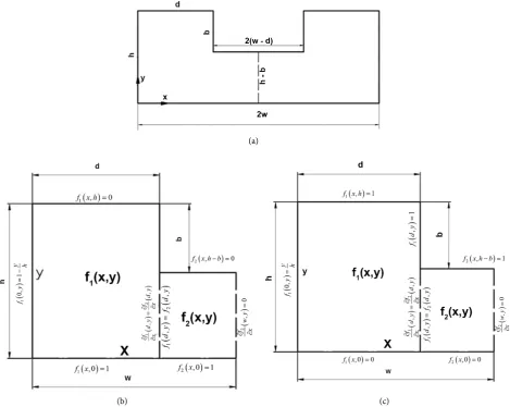
The geometric domain in Figure 1(a) is a concave geometric pattern. The outer dimension of the domain is 2w h× _{, and there is a concave, whose dimension is}

(

)

2 w d b− × . The present research considered two cases of the concave domain. In the first case, the boundary conditions of the bottom is 1, and the boundary conditions of the top is 0. That is to say, the high potential is in the bottom of the domain. And the low potential is in the top of the domain. In the second case, the boundary conditions of the bottom is 0, and the boundary conditions of the top is 1. That is to say, the high potential is in the top of the domain. And the low potential is in the bottom of the domain.

The analysis of boundary conditions on Case 1:

(3)

DOI: 10.4236/wjet.2018.62019 306 World Journal of Engineering and Technology (a)

[image:3.595.64.534.74.448.2]

(b) (c)

Figure 1. (a) The figure of the concave domain; (b) The geometric pattern for the L-shape domain—Case 1; (c) The geometric pattern for the L-shape domain—Case 2.

The governing equation for the region is expressed with Laplace equation:

( )

2_{f x y}_, ₀

∇ = ₍₁₎

The L-shape region is composed of two rectangles; the governing equation for the left one is:

( )

2

1 , 0

f x y

∇ = (2) The boundary conditions for Equation (2) are:

( )

1 ,0 1

f x =

( )

1 , 0

f x h =

( )

1 0, 1

y

f y

h

= − (3)

And the governing equation for the right rectangle is:

(

)

2

2 , 0

f x y

(4)

The boundary conditions for Equation (4) are:

( )

2 ,0 1

f x =

(

)

2 , 0

f x h b− =

(

)

2 _, ₀

f w y x

∂ ₌

∂ (5)

With the boundary conditions Equations (3) and (5), the analytical solution to Equation (2) is f x y1

( )

, , and to Equation (6) is f x y2

( )

, . They are as

fol-lows:

(

)

(

)

(

( ) ( )

)

1 , 1 nsin n e nx d e nx d

n

y

f x y A y

h

α α

α − + − −

= − +

∑

− (6)

(

)

(

)

(

( 2 ) ( )

)

2 , 1 msin m e mx w d e mx d

m

y

f x y B y

h b

β β

β − + − −

= − + +

−

∑

(7)

where the eigenvalues are:

π n h α = π m h b β =

− (8)

Other boundary conditions for governing equations are:

(

)

1 , 0

f d y = ; h b y h− ≤ ≤ ₍₉₎

We choose N points along the boundary at x = d, y ih Ni= and truncate An

to N terms and Bm to M terms, where M =int 1

(

−b h

)

. Substitute the

boun-dary condition into Equation (6), and the following equation can be obtained:

(

)(

2

)

sin e d 1 i 1

n n i

n

y

A y

h

α

α − _{− =} ₋

∑

(10)

i = M + 1 to N

Next, the solutions to the two regions of the L-shape domain can be matched along the common boundary conditions [9]. The conditions can be expressed as:

(

)

(

)

1 , 2 ,

f d y = f d y _,0≤ < −y h b₍₁₁₎

(

)

(

)

1 , 2 ,

f d y f d y

x x

∂ ∂

=

∂ ∂ , 0≤ < −y h b (12)

Substitute the boundary condition into Equations (6)-(7) and can obtain the following equations:

(

)

(

)

(

)

(

( )

)

(

)

2 2

sin e 1 sin 1 e

1

m

w d

d i

n n i m m i

n m

by

A y B y

h h

β α

α − _{− −} β ₊ − − ₌

−

∑

(13)

i = 1 to M

(

)

(

2

)

(

)

(

2( )

)

sin 1 e d sin e w d m 1 0

n n n i m m m i

n A y m B y

β α

α α _{− −} − ₋ β β − − _{− =}

∑

(14)

i = 1 to M

(5)

(

)

1 2

0 0 0

1 d h _{d d} w h b _{d d}

mean

d

f f y x f y x

hw b w d

−

 

= _ + _

− − _

∫ ∫

_ (15)

Integrating Equation (15) can obtain the following equation:

(

)

(

)

(

)

(

)

( ) 2 2 2 2

1 _2e _e ₁

2

cos 1 e 1

d d n mean n w d m m

hw b d w A

f

hw b w d

B _{h b}

α α β α β β − − − − + −  =  + − − − − _    + _ − − _{ } − _ 

∑

(16)

The analysis of boundary conditions on Case 2:

The geometric domain is also a concave domain. The outer dimension of the domain is 2w h× , and there is a concave, whose dimension is 2

(

w d b−

)

× . The boundary condition of the bottom is 0, and the condition of the top is 1. The L-shape region, in Figure 1(c) is composed of two rectangles.

The governing equation for the left rectangle is:

( )

2

1 , 0

f x y

∇ = (17) The boundary conditions for Equation (17) are:

( )

1 ,0 0

f x =

( )

1 , 1

f x h =

( )

1 0, y

f y

h

= (18) And the governing equation for the right rectangle is:

(

)

2

2 , 0

f x y

∇ = ₍₁₉₎

The boundary conditions for Equation (19) are:

( )

2 ,0 0

f x =

(

)

2 , 1

f x h b− =

(

)

2 _, ₀

f w y x

∂ ₌

∂ (20)

With the boundary conditions Equations (18) and (20), the analytical solution to Equation (17) is f x y1

( )

, , and to Equation (19) is f x y2

( )

, . They are as

fol-lows:

(

)

(

)

(

( ) ( )

)

1 , nsin n e nx d e nx d

n

y

f x y C y

h

α α

α − + − −

= +

∑

− (21)

(

)

(

)

(

( 2 ) ( )

)

2 , msin m e mx w d e m x d

m

y

f x y D y

h b

β β

β − + − −

= + +

−

∑

(22)

where the eigenvalues are:

π n h α = π m h b β =

(6)

Other boundary conditions for governing equations are:

(

)

1 , 1

f d y = ; h b y h− ≤ ≤ ₍₂₄₎

Substitute the boundary condition into Equation (21), and the following equa-tion can be obtained:

(

)

(

2

)

sin 1 e d 1

n n i

n

y

C y

h

α

α ₋ − _{= −}

∑

(25)

i = M + 1 to N

Next, the solutions to the two regions of the L-shape domain can be matched along the common boundary conditions. The conditions can be expressed as:

(

)

(

)

1 , 2 ,

f d y = f d y , 0≤ < −y h b (26)

(

)

(

)

1 , 2 ,

f d y f d y

x x

∂ ∂

=

∂ ∂ , 0≤ < −y h b (27)

Substitute the boundary condition into Equations (21)-(22), and can obtain the following equations:

(

)(

)

(

)

(

( )

)

(

)

2 2

sin e d 1 sin 1 e w d m i

n n i m m i

n m

by

C y D y

h h b

β α

α − _{− −} β ₊ − − ₌

−

∑

(28)

i = 1 to M

(

)

(

2 )

)

(

)

(

2( )

)

sin 1 e d sin e w d m 1 0

n n n i m m m i

n C y m D y

β α

α α _{− −} − ₋ β β − − _{− =}

∑

(29)

i = 1 to M

The mean value for f x y

( )

, is expressed as:

(

)

1 2

0 0 0

1 d h _{d d} w h b _{d d}

mean

d

f f y x f y x

hw b w d

−

 

= _ + _

− − _

∫ ∫

_ (30)

Integrating Equation (30) can obtain the following equation:

(

)

(

)

(

)

(

)

( ) 2 2 2 2

1 _2e _e ₁

2

cos 1 e 1

d d n mean n w d m m

hw b d w C

f

hw b w d

D _{h b}

α α β α β β − − − − + −  = _ + − − − − _    + _ − − _{ } − _

∑

(31)

3. Numerical Methods

The following steps of numerical methods are estimated by using Visual C++_:

1) Give the constants h, b, w and d.

2) Set N = 29, M =int 1_

(

−b h

)

__and y ih N_i= _,1≤ ≤i N.

3) Equations (10), (13) and (14) are expressed as the linear system of (N + M) equations to solve coefficients An and Bm.

4) Substitute coefficients An and Bm into equations f1, (Equation (6)) and f2

(Equation (7)). This process is repeated at all nodes within the range, i.e.

0≤ ≤y h_, 0≤ ≤x w.

5) Map the f(x,y) on the entire domain.

(7)

7) Repeat the previous methods can estimate the results of Case 2.

4. Results and Discussion

Results and discussion of Case 1:

Figure 2(a) and Figure 2(b) show the contour plot for the domain. Figure 2(a) is a concave (2w = 1.0, h = 0.5). In the figures, w, b, h and d values are dif-ferent. With the boundary condition Equations (3), (5) and governing equation

( )

1 ,

f x y and f x y2

( )

, , the function values distributing from the bottom of the

domain, f = 1.0 to the top, f = 0 gradually decrease. Besides, the bottom of the domain is high potential, e. g. high temperature or high pressure. The top of the concave domain is low potential, e.g. low temperature or low pressure. The fig-ures show the function values distributing from the maximum value of the bot-tom to the minimum value of the top gradually decrease.

Figure 2(c) shows the local function values for the entire domain (x=0 to

2

x= w_, y=0_to y h= _{). As the figure shows, the bottom region has the}

[image:7.595.63.544.386.695.2]

maximum function values, i.e.f = 1.0, and then function values gradually de-crease from the bottom to the top of the concave domain, f = 0.

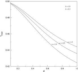
Figure 3 shows the influence of h on the mean values of f x y

( )

, under three different b values (b = 0.25, 0.35 and 0.45). According to Equation (16), the larg-er values of the depth of the concave domain b, and the height of the concave

(a)

(b) (c)

Figure 2. (a) Image for function values, h = 0.5, b = 0.25, d = 0.25, 2w = 1.0; (b) Contour plot for function values, h = 0.5, b = 0.25,

d = 0.25, 2w = 1.0; (c) The distribution of local function values, h = 0.5, b = 0.25, d = 0.25, 2w = 1.0.

0.0 0.1 0.2 0.3 0.4 0.5 0.6 0.7 0.8 0.9 1.0

x

0.0 0.1 0.2 0.3 0.4 0.5

y

0.00 0.05 0.10 0.15 0.20 0.25 0.30 0.35 0.40 0.45 0.50 0.55 0.60 0.65 0.70 0.75 0.80 0.85 0.90 0.95 1.00

0.0 0.1 0.2 0.3 0.4 0.5 0.6 0.7 0.8 0.9 1.0

x 0.0

0.1 0.2 0.3 0.4 0.5

(8)

[image:8.595.163.440.71.333.2]

Figure 3. Mean function values for w = 0.5, d = 0.25—effect on values of h.

Figure 4. Mean function values for h = 1.0, d = 0.3—effect on values of d.

domain h will influence the coefficient An and Bm, and then the mean values of

mean

[image:8.595.159.435.366.619.2]

(9)

DOI: 10.4236/wjet.2018.62019 312 World Journal of Engineering and Technology (a)

[image:9.595.60.542.68.424.2]

(b) (c)

Figure 5. (a) Image for function values, h = 0.4, b = 0.2, d = 0.15, 2w = 0.6; (b) Contour plot for function values, h = 0.4, b = 0.2, d

= 0.15, 2w = 0.6; (c) The distribution of local function values for h = 0.4, b = 0.2, d = 0.15, 2w = 0.6.

Figure 6. Mean function values for w = 0.5, d = 0.25—effect on values of h.

0.00 0.05 0.10 0.15 0.20 0.25 0.30 0.35 0.40 0.45 0.50 0.55 0.60

x

0.00 0.05 0.10 0.15 0.20 0.25 0.30 0.35 0.40

y

0.00 0.05 0.10 0.15 0.20 0.25 0.30 0.35 0.40 0.45 0.50 0.55 0.60 0.65 0.70 0.75 0.80 0.85 0.90 0.95 1.00

0.00 0.05 0.10 0.15 0.20 0.25 0.30 0.35 0.40 0.45 0.50 0.55 0.60 x

0.00 0.05 0.10 0.15 0.20 0.25 0.30 0.35 0.40

[image:9.595.177.421.474.702.2]

(10)

[image:10.595.174.424.72.307.2]

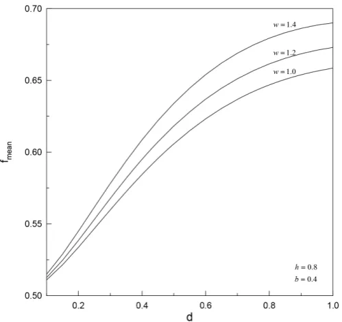
Figure 7. Mean function values for h = 0.8, d = 0.8—effect on values of d.

Figure 4 shows the influence of the values d on the mean values of f x y

( )

,

under three different w values. According to Equations (6), (7) and (16), the larger values of the width of the concave domain w, and the width of the left-top of the concave domain d will also influence the coefficient An and Bm, and then

the mean values of fmean will increase. Besides, observation of the figure shows that the mean values decrease as the values of d increase. And the increase in w leads to an increase in the mean values.

Results and discussions of Case 2:

Figure 5(a) and Figure 5(b) show the contour plot for the concave domain (2w = 0.6, h = 0.4). Basing on the boundary conditions of the case, the function values distributing from the bottom of the domain, f = 0 to the top of the do-main, f = 1.0 gradually increase.

Figure 5(c) shows the local function values for the entire domain (x=0 to

2

x= w,y=0 to y h= _{). As the figure shows, the lower region has the}

mini-mum function values, i.e.f = 0, and then function values gradually increase from bottom to the top of the concave, f = 1.0.

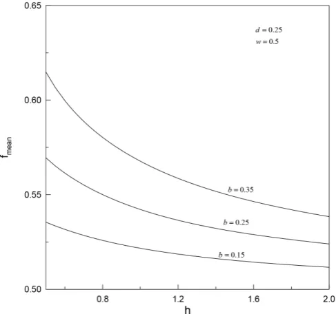
Figure 6 shows the influence of h on the mean values of f x y

( )

, under three different b values. As the figure shows, from h =0.5 to h = 2.0, the mean values of function f x y

( )

, decrease from h = 0.5 to h = 2.0.

Figure 7 shows the influence of the values d on the mean values of f x y

( )

,

under three different w values (w = 1.0, 1.2 and 1.4). Observation of the figure shows that the mean values increase as the values of d increase. And the increase in w leads to an increase in the mean values.

5. Conclusion

(11)

geo-DOI: 10.4236/wjet.2018.62019 314 World Journal of Engineering and Technology

metric domain on the function mean values. Besides, the present paper uses the analytical solution of point match methods and numerical methods which can easily compute coefficient An, Bm, Cn, Dm and function f x y

( )

, .

Acknowledgements

The authors gratefully acknowledge the support provided to this projects by the Ministry of Science and Technology of the Taiwan under Contract Number MOST 106-2221-E-019-062.

References

[1] Alliney, S. (1982) A Numerical Study of Two Dimensional Potential Flows by Boundary and Finite Elements. Applied Mathematical Modelling, 6, 291-298.

https://doi.org/10.1016/S0307-904X(82)80037-1

[2] Rangogni, R. (1986) Numerical Solution of the Generalized Laplace Equation by Coupling the Boundary Element Method and the Perturbation Method. Applied Mathematical Modelling, 10, 266-270.

https://doi.org/10.1016/0307-904X(86)90057-0

[3] Kirkup, S.M. and Henwood, D.J. (1994) An Empirical Error Analysis of the

Boun-dary Element Method Applied to Laplace’s Equation. Applied Mathematical Model-ling, 18, 32-38. https://doi.org/10.1016/0307-904X(94)90180-5

[4] Bailey, R.T., Hsieh, C.K. and Li, H. (1995) Grid Generation in Two Dimensions Using the Complex Variable Boundary Element Method. Applied Mathematical Modelling, 19, 322-332. https://doi.org/10.1016/0307-904X(95)00008-8

[5] Wang, C.Y. (1994) Diffusion across a Corrugated Saw-Tooth Plate. Mechanics Re-search Communications, 116, 233-237.

[6] Chen, J.T. and Chen, K.H. (1998) Analytical Study and Numerical Experiments for Laplace Equation with Overspecified Boundary Conditions. Applied Mathematical Modelling, 22, 703-725. https://doi.org/10.1016/S0307-904X(98)10054-9

[7] Gavete, L., Gavete, M.L. and Benito, J.J. (2003) Improvements of Generalized Finite

Difference Method and Comparison with Other Meshless Method. Applied

Ma-thematical Modelling,27, 831-847. https://doi.org/10.1016/S0307-904X(03)00091-X [8] Nyambuya, G.G. (2015) Four Poisson-Laplace Theory of Gravitation (I). Journal of

Modern Physics, 6, Article ID: 58605, 11 p.

[9] Hu, H.P. (2015) The Two-Dimensional Analysis of Laminar Flow Between the