Risk Evaluation of Dynamic Alliance Based on Fuzzy
Analytic Network Process and Fuzzy TOPSIS
Xiaoguang Zhou1,2, Mi Lu2
1Dongling School of Economics and Management, University of Science and Technology Beijing, Beijing, China; 2Department of
Electrical and Computer Engineering, Texas A&M University, College Station, USA. Email: [email protected], [email protected]
Received May 25th,2012; revised June 23rd, 2012; accepted July 4th, 2012
ABSTRACT
Dynamic alliance formations have increased dramatically over the past decade for its adaptation to environmental change and market competition. However, many fail, while an even greater proportion perform poorly. The risk analy-sis of dynamic alliance will help enterprises to choose a coalition partner and make a reasonable benefit allocation plan. It’s also good for reducing the risk and keeping the stability of the alliance. Based on the interaction and feedback rela-tionships between criteria and/or indices, an index system for evaluating the risk of dynamic alliance is developed. With the information uncertainty and inaccuracy being considered, a new hybrid model based on fuzzy analytic network process (FANP) and fuzzy technique for order performance by similarity to ideal solution (TOPSIS) is proposed. The local weights of criteria and indices are obtained by fuzzy preference programming (FPP), and the comprehensive weights are derived by FANP. According to fuzzy TOPSIS, an optimal alternative is chosen by the closeness coefficient based on the shortest distance from the positive and the farthest distance from the negative ideal solutions. Finally, a numerical case is given by the proposed method.
Keywords: Fuzzy Analytic Network Process; TOPSIS; Dynamic Alliance; Risk Evaluation
1. Introduction
With the rapidly increasing competitiveness in global, enterprise cooperation is necessary in order to meet the market’s requirements for quality, responsiveness, and customer satisfaction. As a result, dynamic alliance, de- fined as voluntary interfirm cooperative arrangements, has become a noteworthy trend in recent years. However, despite the growing numbers and increasing significance of dynamic alliance, many fail, while an even greater proportion perform poorly. Recent estimates put the fail- ure rate of alliances between 60% and 70%, suggesting firms that pursue alliances are more likely than not to fail [1]. Although such failures may be for many interrelated reasons—and may be defined in various ways—two common causes are poor partner selection and poor alli- ance management [2]. Li and Liao [3] pointed out that despite many problems on dynamic alliance, such as part- ner selection, operation management, information ex-changes and their standards, etc. have been investigated, and the risk management of dynamic alliance has not re- ceived deserved attention until now. This article focuses on risk evaluation, which is the most important phase of risk management for dynamic alliance.
Venkatesh et al. [4] investigated the dynamic aspects
of a co-marketing alliance and offered guidelines to es- tablish profitable and self-sustaining alliances. They ex- amined two questions. First, under what market-driven characteristics should either brand manufacturer forge or sustain the alliance. Second, what product market char- acteristics should the alliance promoter seek or alter to increase its payoffs from the alliance. Das and Teng [5] proposed a model of dynamic alliance that has manage- rial risk perception as its core. The model consists of the following parts: the antecedents of risk perception, rela- tional risk and performance risk, risk perception and structural preference, and the resolution of preferences. Rosenkranz and Schmitz [6] explored the dynamic evo- lution of property rights regimes in R&D alliances using the incomplete contract approach, and characterized dif- ferent scenarios in which the optimal ownership structure may change over time due to a trade-off between induc- ing know-how disclosure and ensuring maximum effort. Ip et al. [7] pointed out that minimizing risk in partner
discussed three kinds of learning in alliances—namely, content, partner-specific, and alliance management—and the saliencies and implications of particular types of learning in different alliance stages. Huang et al. [9] pro-
posed a fuzzy synthetic evaluation embedded nonlinear integer programming model of risk programming for dynamic alliance and presented a tabu search algorithm for the model. Delerue and Simon [10] pointed out that cross-cultural interactions were growing at an exponen- tial pace. Consequently, it was becoming important to be aware of the existence and precise nature of cultural dif- ferences in risk perceptions. Huang et al. [11] introduced
a Distributed Decision Making (DDM) model for the risk management of dynamic alliance. The model has two levels, which describe the decision processes of the owner and the partners of the dynamic alliance, respectively. It can be regarded as a combination of both the top-down and bottom-up approaches for risk management of the dynamic alliance. Lee et al. [12] demonstrated the locus
of dynamic knowledge articulation and dynamic capa-bilities development by investigating drivers of dynamic learning in service alliance firms, etc.
However, the interaction and feedback relationships between criteria and/or indices are not completely con- sidered in the existing research literatures. What’s more, during the risk evaluation process of dynamic alliance, there are lots of uncertainty and fuzzy information, the crisp pairwise comparison seems to be insufficient and imprecise to capture the right judgments of decision- makers. Therefore, Zhou and Song proposed a FANP- based method to make up for the deficiency in the con- ventional risk assessment process [13].
The objective of this paper is to present a new hybrid model based on FANP and fuzzy TOPSIS for risk evaluation of dynamic alliance. According to FANP, the weights of criteria/indices are derived. The candidates can be ranked based on their relative closeness according to fuzzy TOPSIS. TOPSIS compromise solution is quite similar to what happens during the decision making process in risk evaluation: most of the time, the best so- lution is not reached since the criteria are not in agree- ment, some must be maximized and others minimized. Such an ANP/AHP-based TOPSIS driven by a set of weighting factors associated with the selected criteria has been proven effective for final ranking via an iterative procedure [14].
2. Preliminary Knowledge
2.1. Triangular Fuzzy NumberA fuzzy set is a class of objects with a continuum of grades of membership. Such a set is characterized by a membership function, which assigns to each object a grade of membership ranging between zero and one. A
triangular fuzzy number (TFN) is denoted simply as (l, m, u). The parameters l, m and u, respectively, denote the
smallest possible value, the most promising value, and the largest possible value that describe a fuzzy event. Each TFN has linear representations on its left and right side such that its membership function can be defined as
,, ,0, otherwise.
M ,
x l m l l x m u x u x u m m x u
(1)
2.2. Fuzzy Analytic Network Process
The Analytic Network Process (ANP), introduced by Saaty [15], is a generalization of the Analytic Hierarchy Process (AHP). The basic assumption of the AHP is that the decision-making problem can be decomposed in a linear top-to-bottom form as a hierarchy, where the upper levels are functionally independent from all lower levels, and the elements in each level are also independent. However, many decision-making problems cannot be structured hierarchically, or there would have strong in- teractions and dependencies between criteria and/or in- dices. The resulting analytic network process provides a framework for dealing with decision-making problems within which assumptions about dependencies between criteria and alternatives are unnecessary.
AHP/ANP has been proposed as a suitable multi-cri- teria decision analysis tool [16,17]. However, the AHP/ ANP-based decision model seems to be ineffective in dealing with the inherent fuzziness or uncertainty for judgment during the pairwise comparison process. Al- though the use of the discrete scale of 1 - 9 to represent the verbal judgment in pairwise comparisons has the ad- vantage of simplicity, it does not take into account the uncertainty associated with the mapping of one’s percep- tion or judgment to a number. In real-life decision-mak- ing situation, the decision makers or stakeholders could be uncertain about their own level of preference, due to incomplete information or knowledge, complexity and uncertainty within the decision environment. Such condi- tions will occur when evaluating the risk of dynamic al- liance. Therefore, it’s more appropriate to make risk management plan under fuzzy condition.
with a Lambda-Max method, which is the direct fuzzifi- cation of the well-known kmax method. Mikhailov [23] de- veloped a fuzzy preference programming method, which also derives crisp weights from fuzzy comparison matri-ces. Srdjevic [24] proposed a multi-criteria approach for combining prioritization methods within the AHP, in-cluding additive normalization, eigenvector, weighted least- squares, logarithmic least-squares, logarithmic goal pro-gramming and fuzzy preference propro-gramming. Wang et al. [25] presented a modified fuzzy logarithmic least
square method. Yu and Cheng [26] developed a multiple objective programming approach for the ANP to obtain all local priorities for crisp or interval judgments at one time. Huo et al. [27] proposed new parametric
prioritiza-tion methods (PPMs) to determine a family of priority vectors in AHP, etc.
2.3. Fuzzy Preference Programming Method
FPP method, as a reasonable and effective means, is adopted in this study. This method can acquire the con- sistency ratios of fuzzy pairwise comparison matrices without conducting an additional study, and the local weights can be easily solved with the help of a Matlab program. The stages of Mikhailov’s fuzzy prioritization approach are as follows [23].
Consider a prioritization problem with n elements,
where the pairwise comparison judgments are repre- sented by normal fuzzy sets or fuzzy numbers. Suppose the decision-maker can provide a set F
aij of
1 2
mn n fuzzy comparison judgments, i = 1, 2, ···, n − 1; j = 2, 3, ···, n; j > i, represented as triangular fuzzy
numbers . The problem is to derive a
crisp priority vector 1 2 , such that the priority ratios wi/wj are approximately within the scopes
of the initial fuzzy judgments, or
, ,ij ij ij ij
ã l m u
, , , T nw w w w
, i ij ij j w l w
u (2)
where the symbol “ ” denotes the statement “fuzzy less or equal to”.
Each crisp priority vector w satisfies the double-side
inequality (2) with some degree, which can be measured by a membership function, linear with respect to the un-known ratio wi/wj,
, ,
, .
i j ij i
ij
ij ij j
i ij
j ij i j
i ij
ij ij j
w w l w
m
m l w
w u
w u w w w
m
u m w
(3)
Taking into consideration the specific form of the membership functions (3), the prioritization problem can be further transformed into a bilinear program of the type
1 max 0, 0,1, 0, 1,2, , .
1,2, , 1; 2,3, , ; .
ij ij j i ij j
ij ij j i ij j
n
k k
k
m l w w l w
u m w w u w
w w k n
i n j n j i
(4)The optimal solution to the non-linear problem (w*,*)
might be obtained by employing some appropriate nu- merical method for non-linear optimization. The optimal value *, if it is positive, indicates that all solution ratios completely satisfy the fuzzy judgment, which means that the initial set of fuzzy judgments is rather consistent. A negative value of * shows that the solutions ratios ap- proximately satisfy all double-side inequalities (2). There- fore, the optimal value * can be used for measuring the consistency of the initial set of fuzzy judgments.
3. Proposed Risk Evaluation of Dynamic
Alliance Framework
This study proposes a novel hybrid analytic approach based on the FANP and fuzzy TOPSIS methodologies to assist in risk evaluation of dynamic alliance. We first identify the evaluation criteria, and present the evaluation model in the following subsections.
3.1. Index system of Risk Evaluation
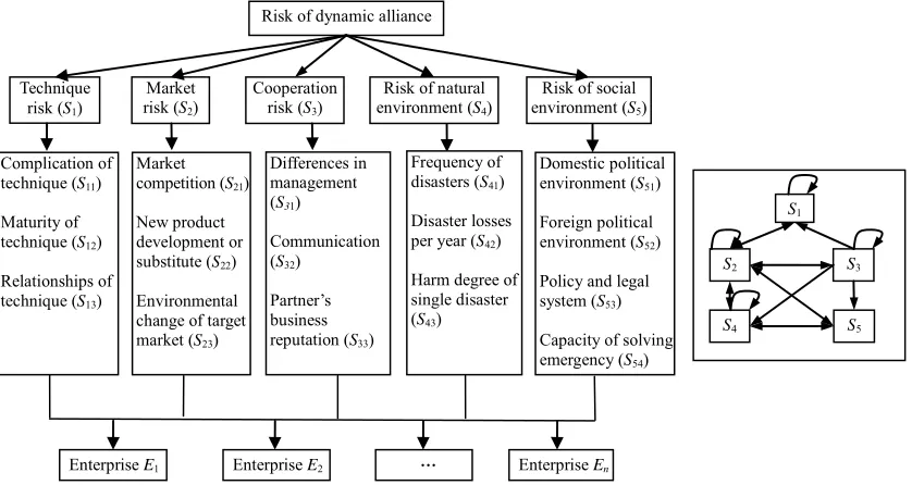
With the risk sources of dynamic alliance being consi- dered, an index system of risk evaluation for dynamic alliance is presented. The index system is made up of five parts: technique risk, market risk, cooperation risk, risk of natural environmental and risk of social environ- mental, as shown in Figure 1.
Technique risk and cooperation risk belong to inner risk. On the contrary, market risk, risk of natural envi- ronment and social environment belong to outer risk. Technique risk is caused by the technique of partners, including complication of technique, maturity of tech- nique and relationships of technique. Cooperation risk is due to the differences in management, communication and partner’s business reputation in an alliance. Market risk is caused by the situation of market competition, new product development or the appearance of substitute and environmental change of target market. The risk of natural environment is due to the earthquakes, droughts, and other natural risk, including frequency of disasters, disaster losses per year and harm degree of single disas- ter. The risk of social environment is caused by war, pol- icy and legal system, and so on, including domestic po- litical environment, foreign political environment, policy and legal system and capacity of solving emergency.
[image:3.595.101.255.630.695.2]Risk of dynamic alliance
Technique risk (S1)
Risk of social environment (S5)
Market risk (S2)
Cooperation risk (S3)
Enterprise E1 Enterprise E2 …
Risk of natural environment (S4)
Enterprise En
S1
S2 S3
S4 S5
Domestic political environment (S51)
Foreign political environment (S52)
Policy and legal system (S53)
Capacity of solving emergency (S54)
Frequency of disasters (S41)
Disaster losses per year (S42)
Harm degree of single disaster (S43)
Differences in management (S31)
Communication (S32)
Partner’s business reputation (S33)
Market competition (S21)
New product development or substitute (S22)
Environmental change of target market (S23)
Complication of technique (S11)
Maturity of technique (S12)
[image:4.595.91.510.88.311.2]Relationships of technique (S13)
[image:4.595.309.538.364.540.2]Figure 1. Index system of risk evaluation of dynamic alliance.
Table 1. Linguistic scales for relative importance of pair-wise comparison.
between criteria and/or indices are being considered. Generally, if market risk (S2) has an effect on technique risk (S1), then a line with arrow from S1 to S2 is added. If the sub-criteria of market risk (S2) have interaction itself, then S2 is inner dependence, and an arc with arrow is added to S2.
Linguistic scales for importance
Triangular fuzzy numbers
Triangular fuzzy reciprocal numbers
Equally important (EI) (1, 1, 1) (1, 1, 1)
Intermediate 1 (IM1) (1, 2, 3) (1/3, 1/2, 1)
Moderately important (MI) (2, 3, 4) (1/4, 1/3, 1/2)
Intermediate 2 (IM2) (3, 4, 5) (1/5, 1/4, 1/3)
Important (I) (4, 5, 6) (1/6, 1/5, 1/4)
Intermediate 3 (IM3) (5, 6, 7) (1/7, 1/6, 1/5)
Very important (VI) (6, 7, 8) (1/8, 1/7, 1/6)
Intermediate 4 (IM4) (7, 8, 9) (1/9, 1/8, 1/7)
Absolutely important (AI) (9, 9, 9) (1/9, 1/9, 1/9)
3.2. Fuzzy Linguistic Variables
During the process of risk evaluation, experts tend to specify their preferences in the form of natural language expressions. The fuzzy linguistic variables are variables reflect different aspects of human language. Their values represent the range from natural to artificial language.
When the values of a linguistic factor are being reflec- ted, the resulting variable must also reflect appropriate modes of change. Moreover, variables describing a hu- man word or sentence can be divided into numerous lin- guistic criteria, such as equally important, moderately important, important, very important and absolutely im- portant. For the purposes of the present study, two 9- point scales are proposed for relative importance of pair- wise comparison and rating the candidates, as shown in Tables 1 and 2.
Table 2. Linguistic scales for rating the candidates. Linguistic scales for positive
sub-factors
Triangular fuzzy numbers Absolutely high (AH) (0.8, 0.9, 1)
Very high (VH) (0.7, 0.8, 0.9)
High (H) (0.6, 0.7, 0.8)
Medium high (MH) (0.5, 0.6, 0.7)
Fair (F) (0.4, 0.5, 0.6)
Medium low (ML) (0.3, 0.4, 0.5)
Low (L) (0.2, 0.3, 0.4)
Very low (VL) (0.1, 0.2, 0.3)
Absolutely low (AL) (0, 0.1, 0.2)
3.3. FANP-Based Approach
The weights of criteria and sub-criteria are obtained based on FANP. The FANP-based approach is proposed step- by-step as follows.
[image:4.595.309.536.569.737.2]of dynamic alliance; the second level is criteria, includ- ing technique risk, market risk, cooperation risk, risk of natural environment and risk of social environment; the third level is sub-criteria, including 16 indicators; the lowest one is candidates.
Step 2. Establish pairwise comparison matrices by the decision committee using the linguistic scales given in Table 1. The decision makers are asked to respond to a series of pairwise comparison with respect to the dimen- sions/attributes-enablers levels in Figure 1. For example, the market competition (S21) and the new product deve- lopment or substitute (S22) are compared using the ques- tion “How important is the market competition when it is compared with the new product development or substi- tute at the dimension of market risk?” and the answer is “intermediate important (IM1)”, so this linguistic scale is placed in the relevant cell against the triangular fuzzy numbers (1, 2, 3). All the fuzzy evaluation matrices are produced in the same way.
Step 3. Calculate the local weights and consistency ra- tios. According to formulation (4), local weights and con- sistency ratios of the criteria and sub-criteria are calcu-lated by FPP method with the help of Matlab.
Step 4. Construct an unweighted supermatrix on the basis of the interdependencies in the network. The super- matrix is a partitioned matrix, where each submatrix is composed of a set of relationships between criteria and indices. Three types of relationships may be encountered in this model: independence from succeeding compo- nents, interdependence among components and interde- pendence between levels of components.
Step 5. Derive a weighted supermatrix. Because in each column it consists of several eigenvectors each of them sums to one and hence the entire column of the matrix may sum to an integer greater than one, the un- weighted supermatrix needs to be stochastic to derive the weighted supermatrix.
Step 6. Generate a limit supermatrix by raising the weighted supermatrix to powers until it converges.
lim t. t
W W
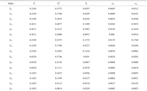
(5) Step 7. Obtain the global weight. A global weight of each index can be computed by multiplying the local weight of the criterion level indicator, the weight of in- dependent sub-criterion and the weight of interdependent sub- criterion.
,
D I
ij i ij ij
w P A A (6) where wijis the comprehensive weight, Pi is relative im-
portance weight of dimension i on final goal; AijD, rela-
tive importance weight for attribute-enabler j of dimen-
sion i, and for the dependency (D) relationships within
attribute-enabler’s component level; I ij
A , stabilized rela- tive importance weight for attribute-enabler j of dimen-
sion i, and for the independency (I) relationships within
attribute-enabler’s component level.
3.4. Fuzzy TOPSIS Approach
TOPSIS method is a classical approach to multi-attribute or multi-criteria decision making problems, which was first proposed by Hwang and Yoon [28] and expanded by Chen and his cooperators [29]. It is a practical and useful technique for ranking and selection of a number of ex- ternally determined alternatives through distance mea- sures. The foundational principle is that the chosen al- ternative should have the shortest distance from the posi- tive ideal solution and the farthest distance from the negative ideal solution.
In the traditional TOPSIS, the performance ratings and the weights of the criteria are given as crisp values. Un- der many conditions, crisp values are inadequate to model real world situations because human judgment and preference are often ambiguous and cannot be estimated with exact numerical values. To resolve the ambiguity frequently existing in the process of judgment and evaluation, fuzzy sets were applied to establish a proto- type fuzzy TOPSIS [30,31].
According to fuzzy TOPSIS, the candidates can be ranked based on their relative closeness. The process is proposed step-by-step as follows.
Step 8. Evaluate the ratings of candidates by the deci- sion committee using the linguistic variables given in Table 2. Assume that a decision group has K persons,
and then the ratings of candidates with respect to each criterion can be calculated as
1 2
1 K
ij ij ij ij
x x x x
k
, (7)
where K ij
x is the rating of the kth decision maker, and xij
can be described by triangular fuzzy numbers, such as xij
= (aij, bij, cij).
Step 9. Construct a fuzzy decision matrix by convert-ing the lconvert-inguistic scales into triangular fuzzy numbers according to Table 2.
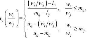
Step 10. Normalize the fuzzy decision matrix. As there are benefit criteria and cost criteria, the fuzzy decision matrices need to be normalized. Given a TFN
ij, ,ij ij
x a b c , in reference to the fuzzy TOPSIS method developed by Chen [28], the normalized per- formance rating can be calculated by
, , , 1, 2, , ,
ij ij ij
ij B
j j j
a b c
r i n
c c c
jW , (8)
and
, , , 1, 2, , ,
j j j
ij C
ij ij ij
a a a
r i n
c b a
where
max ,
j ij b
c c j ,
min ,
j ij c
a a j ,
with B being the benefit criteria set (the larger ij, the
greater preference), and C being the cost criteria set (the
smaller , the greater preference).
r
ij
Hence, the normalized matrix can be ob- tained.
r
ij n m R r
Step 11. Obtain the deal and negative ideal solutions. The ideal solutions can be defined as:
1,1,1 ,
b;
0, 0, 0 ,
c.A jW A jW
Step 12. Determine the distances between each candi- date and the positive or negative ideal candidate.
By considering the different importance of each crite- rion obtained from FANP method, the weighted distance can be calculated as:
3
21
1
, ,
3 i i
ij x y
i
d N M w N M
, (10)
3
21
1
, ,
3 i i
ij x y
i
D N M w N M
,
(11)where and are the primary and
secondary distant measure, respectively. The distance of each candidate from the ideal alternative can be thereby calculated by
,D N M D
N M ,
2
2
1
1 1 1 1
3
m
i ij ij ij ij
j
d w g h l
2 . (12)
Similarly, the separation from the negative ideal solu-tion is given by
2
2
1
1
0 0 0
3
m
i ij ij ij ij
j
d w g h l
2. (13)Step 13. Calculate the relative closeness *. i RC
* i .
i i i d RC d d
(14) According to the values of , the candidates can be ranked.
*
i RC
4. Case Study
Suppose four spinning mills will form a dynamic alliance through pre-test. The four candidates are recorded as E1, E2, E3 and E4. In order to make a reasonable benefit allo- cation plan and attain a stability of the alliance, a cross- functional decision committee consisting of various de- partments works to evaluate the risk of the four enter- prises, named as D1, D2 and D3. The results will assist in
making benefit allocation plan and risk management as well. The risk evaluating process based on FANP and fuzzy TOPSIS is as follows.
Step 1. With the interaction and feedback relationships between dimensions and/or attribute-enablers being con- sidered, a four-level evaluation index system is presented, as shown in Figure 1.
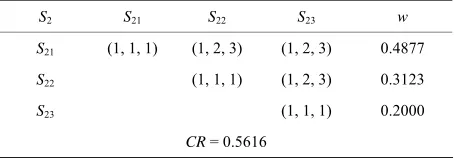
Step 2. Pairwise comparison matrices among dimen- sions and/or attributes are formed by the decision com-mittee using the linguistic scales given in Table 1. For example, Table 3 is the pairwise comparison matrix for market competition (S21), new product development or substitute (S22) and environmental change of target mar- ket (S23) at the dimension of market risk.
Expert opinions will be converted into the correspond- ing triangular fuzzy numbers, as shown in Table 4. All the fuzzy evaluation matrices are produced in the same manner.
Step 3. Local weights of the factors and sub-factors which take part in the second and third levels of the ANP model, provided in Figure 1, are calculated by FPP method. For instance, according to equation (4), the local weights of Table 4 can be obtained by solving the fol- lowing non-linear programming.
2 1 2
2 1 2
3 1 3
3 1 3
3 2 3
3 2 3
1 2 3
1 2 3
max 0; 3 0 0; 3 0 0; 3 0 1;
, , 0.
w w w
w w w
w w w
w w w
w w w
w w w
w w w
w w w
[image:6.595.98.286.319.381.2]; ; ;
Table 3. The comparison matrix at the dimension of market risk using linguistic variables.
S2 S21 S22 S23
S21 EI IM1 IM1
S22 EI IM1
[image:6.595.308.537.551.616.2]S23 EI
Table 4. The comparison matrix at the dimension of market risk using TFNs.
S2 S21 S22 S23 w
S21 (1, 1, 1) (1, 2, 3) (1, 2, 3) 0.4877
S22 (1, 1, 1) (1, 2, 3) 0.3123
S23 (1, 1, 1) 0.2000
[image:6.595.310.537.655.734.2]in Table 8. It can be solved by Matlab, and the optimal solutions
are w1 = 0.4877, w2 = 0.3123, w3 = 0.2000, as shown in Table 4. Consistency index CR is 0.5616, which shows
that the experts’ opinions have a good consistency, and the local weights are acceptable. All the local weights of comparison matrices are calculated in the same way.
Step 11. Positive and negative ideal solutions are de-fined as
1,1,1 ,
b;
0,0,0 ,
c.A jW A jW
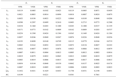
Step 12. According to Equations (12) and (13), the weighted distances of each candidate from FPIS and FNIS can be calculated, as shown in Table 9.
Step 4. According to the interdependencies among di- mensions and attribute-enablers of the ANP model, an
unweighted supermatrix is built, as shown in Table 5. Step 13. According to Equation (14), the relative close- ness of the four enterprises can be calculated by RC1 = 0.8199, RC2 = 0.8221, RC3 = 0.830 and RC4 = 0.7861, as shown in Table 9. Therefore, the risk profile of the four enterprises can be ranked as E3 E2E1 E4, and en-terprise E3 is the best one.
Step 5. The unweighted supermatrix is being random- ized to derive the weighted supermatrix.
Step 6. According to Equation (5), multiplying the weighted supermatrix by itself until the supermatrix’s row values converge to the same value for each column of the matrix, then we choose any column from the steady limit supermatrix as the local weights of the in- terdependency indicators, as shown in Table 6.
The same ranking of the alternatives is drawn as ref- erence [13], but this time the weights are obtained by FANP, and the ranking is determined by the closeness coefficient based on the distances to the positive and negative ideal solutions. It provides a new approach for evaluating the risk of dynamic alliance. As mentioned before, it is more adaptive to the final ranking of the al- ternatives as well.
Step 7. According to Equation (6), the comprehensive weight wij of each index can be calculated, as shown in
Table 7, and ij is the normalized weight of wij.
Step 8. The ratings of the enterprises with respect to each indicator are determined by Table 2.
w
Step 9. To construct fuzzy decision matrix, the linguis- tic scales are converted into triangular fuzzy numbers. According to the formulation (7), the ratings of the can- didates with respect to each criterion can be calculated
5. Conclusion
With the interaction and feedback relationships between criteria and/or indicators being considered, an index system for evaluating the risk of dynamic alliance is Step 10. According to Equations (8) and (9), the nor-
malized fuzzy decision matrix can be acquired, as shown
Table 5. The unweighted supermatrix.
S11 S12 S13 S21 S22 S23 S31 S32 S33 S41 S42 S43 S51 S52 S53 S54
S11 0.0000 0.6667 0.7500 0.5375 0.3070 0.2500 0.0000 0.0000 0.0000 0.0000 0.0000 0.0000 0.0000 0.0000 0.0000 0.0000
S12 0.3333 0.0000 0.2500 0.1700 0.1677 0.5000 0.0000 0.0000 0.0000 0.0000 0.0000 0.0000 0.0000 0.0000 0.0000 0.0000
S13 0.6667 0.3333 0.0000 0.2925 0.5253 0.2500 0.0000 0.0000 0.0000 0.0000 0.0000 0.0000 0.0000 0.0000 0.0000 0.0000
S21 0.3063 0.3063 0.2500 0.0000 0.8000 0.6667 0.5714 0.4000 0.2000 0.2500 0.2500 0.4000 0.5714 0.5714 0.4000 0.1704
S22 0.5270 0.5270 0.5000 0.6667 0.0000 0.3333 0.2857 0.2000 0.4000 0.2500 0.2500 0.2000 0.2857 0.2857 0.2000 0.3003
S23 0.1667 0.1667 0.2500 0.3333 0.2000 0.0000 0.1429 0.4000 0.4000 0.5000 0.5000 0.4000 0.1429 0.1429 0.4000 0.5292
S31 0.5714 0.5000 0.4286 0.5375 0.2500 0.2857 0.0000 0.6667 0.8000 0.2000 0.4000 0.4000 0.5375 0.5375 0.2500 0.1711
S32 0.1429 0.2500 0.1429 0.1700 0.2500 0.1429 0.3333 0.0000 0.2000 0.4000 0.2000 0.2000 0.1700 0.1700 0.2500 0.5361
S33 0.2857 0.2500 0.4286 0.2925 0.5000 0.5714 0.6667 0.3333 0.0000 0.4000 0.4000 0.4000 0.2925 0.2925 0.5000 0.2928
S41 0.0000 0.0000 0.0000 0.5746 0.4000 0.5000 0.0000 0.0000 0.0000 0.0000 0.8333 0.6667 0.2857 0.2857 0.2500 0.5746
S42 0.0000 0.0000 0.0000 0.3143 0.2000 0.2500 0.0000 0.0000 0.0000 0.7500 0.0000 0.3333 0.5714 0.5714 0.5000 0.3143
S43 0.0000 0.0000 0.0000 0.1111 0.4000 0.2500 0.0000 0.0000 0.0000 0.2500 0.1667 0.0000 0.1429 0.1429 0.2500 0.1111
S51 0.0000 0.0000 0.0000 0.2672 0.2222 0.4159 0.0000 0.0000 0.0000 0.2222 0.4159 0.2672 0.0000 0.0000 0.0000 0.0000
S52 0.0000 0.0000 0.0000 0.1399 0.1111 0.1315 0.0000 0.0000 0.0000 0.1111 0.1315 0.1399 0.0000 0.0000 0.0000 0.0000
S53 0.0000 0.0000 0.0000 0.5115 0.2222 0.2263 0.0000 0.0000 0.0000 0.2222 0.2263 0.5115 0.0000 0.0000 0.0000 0.0000
Table 6. The limit supermatrix.
S11 S12 S13 S21 S22 S23 S31 S32 S33 S41 S42 S43 S51 S52 S53 S54
S11 0.0397 0.0397 0.0397 0.0397 0.0397 0.0397 0.0397 0.0397 0.0397 0.0397 0.0397 0.0397 0.0397 0.0397 0.0397 0.0397
S12 0.0249 0.0249 0.0249 0.0249 0.0249 0.0249 0.0249 0.0249 0.0249 0.0249 0.0249 0.0249 0.0249 0.0249 0.0249 0.0249
S13 0.0354 0.0354 0.0354 0.0354 0.0354 0.0354 0.0354 0.0354 0.0354 0.0354 0.0354 0.0354 0.0354 0.0354 0.0354 0.0354
S21 0.1289 0.1289 0.1289 0.1289 0.1289 0.1289 0.1289 0.1289 0.1289 0.1289 0.1289 0.1289 0.1289 0.1289 0.1289 0.1289
S22 0.1091 0.1091 0.1091 0.1091 0.1091 0.1091 0.1091 0.1091 0.1091 0.1091 0.1091 0.1091 0.1091 0.1091 0.1091 0.1091
S23 0.0953 0.0953 0.0953 0.0953 0.0953 0.0953 0.0953 0.0953 0.0953 0.0953 0.0953 0.0953 0.0953 0.0953 0.0953 0.0953
S31 0.1372 0.1372 0.1372 0.1372 0.1372 0.1372 0.1372 0.1372 0.1372 0.1372 0.1372 0.1372 0.1372 0.1372 0.1372 0.1372
S32 0.0727 0.0727 0.0727 0.0727 0.0727 0.0727 0.0727 0.0727 0.0727 0.0727 0.0727 0.0727 0.0727 0.0727 0.0727 0.0727
S33 0.1234 0.1234 0.1234 0.1234 0.1234 0.1234 0.1234 0.1234 0.1234 0.1234 0.1234 0.1234 0.1234 0.1234 0.1234 0.1234
S41 0.059 0.059 0.059 0.059 0.059 0.059 0.059 0.059 0.059 0.059 0.059 0.059 0.059 0.059 0.059 0.059
S42 0.0467 0.0467 0.0467 0.0467 0.0467 0.0467 0.0467 0.0467 0.0467 0.0467 0.0467 0.0467 0.0467 0.0467 0.0467 0.0467
S43 0.0276 0.0276 0.0276 0.0276 0.0276 0.0276 0.0276 0.0276 0.0276 0.0276 0.0276 0.0276 0.0276 0.0276 0.0276 0.0276
S51 0.0296 0.0296 0.0296 0.0296 0.0296 0.0296 0.0296 0.0296 0.0296 0.0296 0.0296 0.0296 0.0296 0.0296 0.0296 0.0296
S52 0.0127 0.0127 0.0127 0.0127 0.0127 0.0127 0.0127 0.0127 0.0127 0.0127 0.0127 0.0127 0.0127 0.0127 0.0127 0.0127
S53 0.0318 0.0318 0.0318 0.0318 0.0318 0.0318 0.0318 0.0318 0.0318 0.0318 0.0318 0.0318 0.0318 0.0318 0.0318 0.0318
[image:8.595.56.540.431.733.2]S54 0.0259 0.0259 0.0259 0.0259 0.0259 0.0259 0.0259 0.0259 0.0259 0.0259 0.0259 0.0259 0.0259 0.0259 0.0259 0.0259
Table 7. Comprehensive weights of the indicators.
Index Pi
D ij
A I
ij
A wij wij
S11 0.2105 0.5375 0.0397 0.0045 0.0512
S12 0.2105 0.1700 0.0249 0.0009 0.0101
S13 0.2105 0.2925 0.0354 0.0022 0.0248
S21 0.4211 0.4877 0.1289 0.0265 0.3015
S22 0.4211 0.3123 0.1091 0.0143 0.1634
S23 0.4211 0.2000 0.0953 0.008 0.0914
S31 0.2105 0.5375 0.1372 0.0155 0.1768
S32 0.2105 0.1700 0.0727 0.0026 0.0296
S33 0.2105 0.2925 0.1234 0.0076 0.0865
S41 0.0526 0.5746 0.059 0.0018 0.0203
S42 0.0526 0.3143 0.0467 0.0008 0.0088
S43 0.0526 0.1111 0.0276 0.0002 0.0018
S51 0.1053 0.2672 0.0296 0.0008 0.0095
S52 0.1053 0.1399 0.0127 0.0002 0.0021
S53 0.1053 0.5115 0.0318 0.0017 0.0195
Table 8. The fuzzy normalized decision matrix.
E1 E2 E3 E4 wij
D1 D2 D3 D1 D2 D3 D1 D2 D3 D1 D2 D3
S11 0.6785 0.7856 0.8928 0.7149 0.8221 0.9293 0.6785 0.7856 0.8928 0.7856 0.8928 1.0000 0.0512
S12 0.7033 0.8144 0.9256 0.7778 0.8889 1.0000 0.7411 0.8522 0.9633 0.6667 0.7778 0.8889 0.0101
S13 0.6898 0.7932 0.8966 0.7932 0.8966 1.0000 0.6546 0.7580 0.8614 0.7239 0.8273 0.9307 0.0248
S21 0.7239 0.8273 0.9307 0.7580 0.8614 0.9648 0.7932 0.8966 1.0000 0.6546 0.7580 0.8614 0.3015
S22 0.7778 0.8889 1.0000 0.7411 0.8522 0.9633 0.7411 0.8522 0.9633 0.7033 0.8144 0.9256 0.1634
S23 0.7203 0.8403 0.9604 0.7599 0.8800 1.0000 0.7599 0.8800 1.0000 0.6807 0.8007 0.9208 0.0914
S31 0.7778 0.8889 1.0000 0.6667 0.7778 0.8889 0.7033 0.8144 0.9256 0.6667 0.7778 0.8889 0.1768
S32 0.7239 0.8273 0.9307 0.7932 0.8966 1.0000 0.6546 0.7580 0.8614 0.7580 0.8614 0.9648 0.0296
S33 0.6898 0.7932 0.8966 0.7580 0.8614 0.9648 0.7932 0.8966 1.0000 0.7239 0.8273 0.9307 0.0865
S41 0.6898 0.7932 0.8966 0.6546 0.7580 0.8614 0.5512 0.6546 0.7580 0.7932 0.8966 1.0000 0.0203
S42 0.5359 0.6431 0.7503 0.7503 0.8574 0.9646 0.6431 0.7503 0.8574 0.7856 0.8928 1.0000 0.0088
S43 0.4802 0.6002 0.7203 0.6807 0.8007 0.9208 0.6002 0.7203 0.8403 0.7599 0.8800 1.0000 0.0018
S51 0.7147 0.8218 0.9290 0.5711 0.6782 0.7854 0.7854 0.8925 0.9997 0.7147 0.8218 0.9290 0.0095
S52 0.7932 0.8966 1.0000 0.6205 0.7239 0.8273 0.6898 0.7932 0.8966 0.6205 0.7239 0.8273 0.0021
S53 0.6330 0.7330 0.8330 0.6670 0.7670 0.8670 0.7000 0.8000 0.9000 0.8000 0.9000 1.0000 0.0195
S54 0.6205 0.7239 0.8273 0.7239 0.8273 0.9307 0.6898 0.7932 0.8966 0.7932 0.8966 1.0000 0.0025
Table 9. Distances to FPIS and FNIS.
E1 E2 E3 E4
VPIS VNIS VPIS VNIS VPIS VNIS VPIS VNIS
S11 0.0119 0.0405 0.0102 0.0423 0.0119 0.0405 0.0071 0.0459
S12 0.0021 0.0083 0.0014 0.0090 0.0018 0.0087 0.0024 0.0079
S13 0.0055 0.0198 0.0033 0.0223 0.0064 0.0189 0.0048 0.0206
S21 0.0580 0.2507 0.0489 0.2610 0.0403 0.2715 0.0773 0.2300
S22 0.0234 0.1460 0.0283 0.1400 0.0283 0.1400 0.0337 0.1339
S23 0.0171 0.0773 0.0142 0.0809 0.0142 0.0809 0.0203 0.0737
S31 0.0254 0.1580 0.0424 0.1384 0.0365 0.1449 0.0424 0.1384
S32 0.0057 0.0246 0.0040 0.0267 0.0076 0.0226 0.0048 0.0256
S33 0.0193 0.0690 0.0140 0.0749 0.0115 0.0779 0.0166 0.0719
S41 0.0045 0.0162 0.0052 0.0155 0.0072 0.0134 0.0027 0.0183
S42 0.0032 0.0057 0.0015 0.0076 0.0023 0.0066 0.0012 0.0079
S43 0.0007 0.0011 0.0004 0.0015 0.0005 0.0013 0.0003 0.0016
S51 0.0019 0.0079 0.0032 0.0065 0.0013 0.0085 0.0019 0.0079
S52 0.0003 0.0019 0.0006 0.0015 0.0005 0.0017 0.0006 0.0015
S53 0.0054 0.0144 0.0048 0.0150 0.0042 0.0157 0.0025 0.0176
S54 0.0007 0.0018 0.0005 0.0021 0.0006 0.0020 0.0003 0.0023
Sij 0.1852 0.8431 0.1829 0.8453 0.1750 0.8551 0.2190 0.8051
RCi 0.8199 0.8221 0.8301 0.7861
[image:9.595.53.539.409.735.2]presented. With the uncertainty and the inaccuracy infor- mation during the evaluation process being considered, a model combining FANP and fuzzy TOPSIS is proposed. The local weights of criteria and indices are calculated by FPP, and the global weights are determined by FANP method. The distances between the candidates and posi- tive ideal solutions or negative ones can be calculated by fuzzy TOPSIS. The rank of the candidates is derived by their relative closeness. A numerical case is given by the proposed method. The risk analysis of dynamic alliance will help enterprises to choose a coalition partner and make a reasonable benefit allocation plan, and it is ad- vantageous in acquiring the stability of the union as well.
6. Acknowledgements
This work was supported by “the Fundamental Research Funds for Chinese Central Universities (No. FRF-BR-11- 009A)”.
REFERENCES
[1] T. P. Munyon, A. A. Perryman, J. P. Morgante and G. R. Ferris, “Firm Relationships—The Dynamics of Effective Organization Alliances,” Organizational Dynamics, Vol. 40, No. 2, 2011, pp. 96-103.
doi:10.1016/j.orgdyn.2011.01.003
[2] S. R. Holmberg and L. J. Cummings, “Building Success- ful Strategic Alliances-Strategic Process and Analytical Tool for Selecting Partner Industries and Firms,” Long Range Planning, Vol. 42, No. 2, 2009, pp. 164-193. doi:10.1016/j.lrp.2009.01.004
[3] Y. Li and X. W. Liao, “Decision Support for Risk Analy- sis on Dynamic Alliance,” Decision Support Systems, Vol. 42, No. 4, 2007, pp. 2043-2059.
doi:10.1016/j.dss.2004.11.008
[4] R. Venkatesh, V. Mahajan and E. Muller, “Dynamic Co- Marketing Alliances—When and Why Do They Succeed or Fail?” International Journal of Research in Marketing, Vol. 17, No. 1, 2000, pp. 3-31.
doi:10.1016/S0167-8116(00)00004-5
[5] T. K. Das and B. S. Teng, “A Risk Perception Model of Alliance Structuring,” Journal of International Manage- ment, Vol. 7, No. 1, 2001, pp. 1-29.
doi:10.1016/S1075-4253(00)00037-5
[6] S. Rosenkranz and P. W. Schmitz, “Optimal Allocation of Ownership Rights in Dynamic R&D Alliances,” Games and Economic Behavior, Vol. 43, No. 1, 2003, pp. 153-173. doi:10.1016/S0899-8256(02)00553-5
[7] W. H. Ip, M. Huang, K. L. Yung and D. W. Wang, “Ge- netic Algorithm Solution for a Risk-Based Partner Selec- tion Problem in a Virtual Enterprise,” Computers & Op- erations Research, Vol. 30, No. 2, 2003, pp. 213-231. doi:10.1016/S0305-0548(01)00092-2
[8] T. K. Das and R. Kumar, “Learning Dynamics in the Al- liance Development Process,” Management Decision, Vol. 45, No. 4, 2007, pp. 684-707.
doi:10.1108/00251740710745980
[9] M. Huang, W. H. Ip, H. M. Yang, X. W. Wang and H. C. W. Lau, “A Fuzzy Synthetic Evaluation Embedded Tabu Search for Risk Programming of Virtual Enterprises,” In- ternational Journal of Production Economics, Vol. 116, No. 1, 2008, pp. 104-114. doi:10.1016/j.ijpe.2008.06.008 [10] H. Delerue and E. Simon, “National Cultural Values and
the Perceived Relational Risks in Biotechnology Alliance Relationships,” International Business Review, Vol. 18, No. 1, 2009, pp. 14-25.
doi:10.1016/j.ibusrev.2008.11.003
[11] M. Huang, F. Q. Lu, W. K. Ching and T. K. Siu, “A Dis- tributed Decision Making Model for Risk Management of Virtual Enterprise,” Expert Systems with Applications, Vol. 38, No. 10, 2011, pp. 13208-13215.
doi:10.1016/j.eswa.2011.04.135
[12] P. Y. Lee, H. H. Chen and Y. H. Shyr, “Driving Dynamic Knowledge Articulation and Dynamic Capabilities De- velopment of Service Alliance Firms,” The Service Indus- tries Journal, Vol. 31, No. 13, 2011, pp. 2223-2242. doi:10.1080/02642069.2010.504820
[13] X. G. Zhou and Y. T. Song, “The Application of Fuzzy Analytic Network Process in Risk Evaluation of Dynamic Alliance,” Proceedings ofIEEE International Conference on Supernetworks and System Management, Shanghai, 29-30 May 2011, pp. 157-162
[14] A. Pires, N. B. Chang and G. Martinbo, “An AHP-Based Fuzzy Interval TOPSIS Assessment for Sustainable Ex- pansion of the Solid Waste Management System in Se- túbal Peninsula, Portugal,” Resources, Conservation and Recycling, Vol. 56, No. 1, 2011, pp. 7-21.
doi:10.1016/j.resconrec.2011.08.004
[15] T. L. Saaty, “Decision Making with Dependence and Feed- back: The Analytic Network Process,” RWS Publications, Pittsburgh, 1996.
[16] Y. P. Ou Yang, H. M. Shieh and G. H. Tzeng, “A VIKOR Technique Based on DEMATEL and ANP for Informa-tion Security Risk Control Assessment,” Information Sci-ence, 2011, in Press. doi:10.1016/j.ins.2011.09.012 [17] N. S. Arunraj and J. Maiti, “Risk-Based Maintenance Po-
licy Selection Using AHP and Goal Programming,” Safety Science, Vol. 48, No. 2, 2010, pp. 238-247.
doi:10.1016/j.resconrec.2011.08.004
[18] P. J. M. Van Laarhoven and W. Pedrycz, “A Fuzzy Ex-ten- sion of Saaty’s Priority Theory,” Fuzzy Sets and Sys-tems, Vol. 11, No. 1-3, 1983, pp. 229-241.
[19] J. J. Buckley, “Fuzzy Hierarchical Analysis,” Fuzzy Sets and Systems, Vol. 17, No. 3, 1985, pp. 233-247.
doi:10.1016/0165-0114(85)90090-9
[20] D. Y. Chang, “Applications of the Extent Analysis Meth- od on Fuzzy AHP,” European Journal of Operational Research, Vol. 95, No. 3, 1996, pp. 649-655.
doi:10.1016/0377-2217(95)00300-2
[21] R. Xu, “Fuzzy Least-Squares Priority Method in the Ana- lytic Hierarchy Process,” Fuzzy Sets and Systems, Vol. 112, No. 3, 2000, pp. 359-404.
doi:10.1016/S0165-0114(97)00376-X
Vol. 120, No. 2, 2001, pp. 181-195. doi:10.1016/S0165-0114(99)00155-4
[23] L. Mikhailov, “Deriving Priorities from Fuzzy Pairwise Comparison Judgements,” Fuzzy Sets and Systems, Vol. 134, No. 3, 2003, pp. 365-385.
doi:10.1016/S0165-0114(02)00383-4
[24] B. Srdjevic. “Combining Different Prioritization Methods in the Analytic Hierarchy Process Synthesis,” Computers & Operations Research, Vol. 32, No. 7, 2005, pp. 1897- 1919. doi:10.1016/j.cor.2003.12.005
[25] Y. M. Wang, T. M. S. Elhag and Z. S. Hua, “A Modified Fuzzy Logarithmic Least Squares Method for Fuzzy Ana- lytic Hierarchy Process,” Fuzzy Sets and Systems, Vol. 157, No. 23, 2006, pp. 3055-3071.
doi:10.1016/j.fss.2006.08.010
[26] J. R. Yu and S. J. Cheng, “An Integrated Approach for Deriving Priorities in Analytic Network Process,” Euro- pean Journal of Operational Research, Vol. 180, No. 3, 2007, pp. 1427-1432. doi:10.1016/j.ejor.2006.06.005 [27] L. A. Huo, J. B. Lan and Z. X. Wang, “New Parametric
Prioritization Methods for an Analytical Hierarchy Proc- ess Based on a Pairwise Comparison Matrix,” Mathema- tical and Computer Modelling, Vol. 54, No. 11-12, 2011, pp. 2736-2749. doi:10.1016/j.mcm.2011.06.062
[28] C. L. Hwang and K. Yoon, “Multiple Attributes Decision Making Methods and Applications,” Springer, Berlin, 1981. doi:10.1007/978-3-642-48318-9
[29] S. J. Chen, C. L. Hwang and F. P. Hwang, “Fuzzy Multi- ple Attribute Decision Making,” Lecture Notes in Eco- nomics and Mathematical System, Vol. 375, 1992, pp. 1- 531.
[30] C. T. Chen, “Extensions of the TOPSIS for Group Deci- sion-Making under Fuzzy Environment,” Fuzzy Sets and Systems, Vol. 114, No. 1, 2000, pp. 1-9.
doi:10.1016/S0165-0114(97)00377-1