Design of Expressway Toll Station Based on Neural Network and Traffic Flow

ISSN Online: 2160-8849 ISSN Print: 2160-8830

DOI: 10.4236/ajor.2018.83013 May 30, 2018 221 American Journal of Operations Research

Design of Expressway Toll Station Based on

Neural Network and Traffic Flow

Yiqian Huang, Liang Chen, Yanwen Xia, Xiuliang Qiu

Abstract

This paper is concerned with the design of expressway toll station problem based on neural network and traffic flow. Firstly, the design of the toll plaza is mainly through analyzing the daily traffic flow, different charging mode of construction cost and waiting time of the United States. Secondly, exploring traffic conditions is divided into two kinds, based on the traffic flow speed-density flow model. Then, a fuzzy-BP neural network model is con-structed, with capacity, cost, and safety factor as the input layers and perfor-mance as the output layer. It is concluded that this scheme will reduce the occurrence of traffic accidents, so it is desirable. Considering that the increase in unmanned vehicles will lead to an increase in safety performance, we in-crease the number of electronic toll stations to improve security performance and reduce the occurrence of traffic accidents.

Keywords

Toll Station, Traffic Flow, Fuzzy-BP Neural Network

1. Background

With the development of highway construction and the growth of automotive bases, holiday travel trends will lead to a surge in passenger traffic. At this time, if we do not limit the high-speed traffic, it will not only seriously affect the oper-ational efficiency of the expressway, but also bring about great security risks. Therefore, we must take measures to ensure the number of peak traffic flows and create a good high-speed environment.

Nowadays, many high-speed toll stations use card charges to collect high fees. In most cases, the toll collection station’s card charge is perpendicular to the freeway. When a car enters a toll booth, it passes through a wide road and How to cite this paper: Huang, Y.Q.,

Chen, L., Xia, Y.W. and Qiu, X.L. (2018) Design of Expressway Toll Station Based on Neural Network and Traffic Flow. Ameri-can Journal of Operations Research, 8, 221-237.

https://doi.org/10.4236/ajor.2018.83013

Received: March 27, 2018 Accepted: May 27, 2018 Published: May 30, 2018

Copyright © 2018 by authors and Scientific Research Publishing Inc. This work is licensed under the Creative Commons Attribution International License (CC BY 4.0).

DOI: 10.4236/ajor.2018.83013 222 American Journal of Operations Research quickly enters a toll booth, such as a fan. In the United States, the proportion of toll roads is very small, less than 4% of the total length of roads, mainly in the east, and Americans often call highway. However, the current trend is that road tolls are gradually increasing. IBTTA’s 2015 annual expense report shows that the toll roads are relatively safe, and the accident rate without toll roads is almost 3 times that of toll roads [1].

2. Basic Assumption

1) Except for traffic, cost, waiting time, number of vehicles and other factors, other factors are ignored.

2) The car runs at a constant speed of 100 km/h.

3) No accidents occurred on the traffic highway. For example, the charging system will not cause service interruption.

4) There is no difference between lanes. The type of car is basically the same.

3. Queuing Model Based on Poisson Distribution

3.1. Model Principle (Table 1)

Set N t

( )

(

)

[

)

(

)

n

P t t as the probability of n cars arrived in time interval

[

)(

)

(

)

{

( )

( )

}

(

)

n

P t t =P N t −N t =n t >t n≥ _{. (1)}

when P t tn

(

)

1) Without overlap the time interval of car to several independent of each other, we call this property has no aftereffect.

2) For sufficiently small Δt, the probability of a car arriving has nothing to do with t in the time interval

[

)

(

)

( )

1 ,

P t t+ ∆ = ∆ + ∆t

λ

when ∆ →t 0_, o t

( )

λ

constant, it says the probability of a car’s arriving, is the probabilistic strength. 3) For sufficiently small Δt, within time interval there are two or more than two cars arrive rarely and that can be ignored. So:

(

)

( )

2 n ,

n P t t t o t

∞

=

+ ∆ = ∆

∑

Under the condition of the above, we study the number of arriving cars to get a probability distribution.

By the conditions of 2, we can always take time from 0, and shorthand

( )

( )

P t =P t .

By the conditions 1 and 2, we say:

(

)

( ) ( )

0 0 0

DOI: 10.4236/ajor.2018.83013 223 American Journal of Operations Research

Table 1. Symbol table.

Variable Description

Model 1

h Boundary value every day

a Traffic volume every minute

λ Toll station of each traffic volume every minute (=a/B) mu The number of the cars detected every minute

Q

L The number of car waiting

S

L The number of car waiting and paying Model 3

F Maximum braking force

m Quality of vehicle

c Ratio coefficient

v Speed

2

d Travel distance

Model 4

K Traffic density

Ф Traffic flow

λ Multiple lanes

f

v Speed smoothly

f

K Congestion state

Model 5

i Unit

X Input vector

Y Output vector

ij

O The output of unit

ij

W Network weights

pj

T Expected output

δ Error signal

i

θ Threshold

(

)

( ) ( )

0 , 1,2,

n

n n k k

k

P t t P− t P t n

=

+ ∆ =

∑

By the conditions 1 and 2, we say:

( )

( )

0 1

P ∆ = − ∆ + ∆t

λ

We come into the conclusion,

(

)

( )

_{( ) ( )}

0 0

0

P t t P t o t

P t

t

λ

+ ∆ − ∆

= − +

∆ ∆ . (7)

(

)

( )

_{( )}

_{( ) ( )}

1

n n

n n

P t t P t o t

P t P t

t

λ

λ

+ ∆ − ∆

= − + +

DOI: 10.4236/ajor.2018.83013 224 American Journal of Operations Research In this above, we take the limit of the tending to 0, when we assume that the function of the design guide, get a system of differential equations:

( )

_{( )}

t = −

λ

( )

_{( )}

_{( )}

P t P t n

t = −

λ

λ

( )

( ) (

)

( )

0 e t

P t ₌ −λ _{, and then take}

( )

( )

n n

P t U t₌ −λ _{again, we can get}

_{( )}

U t and the differential equations that U tn

( )

( )

_{( )}

U t n

t =

λ

( )

( )

0 1, n 0

U t = U t = . (12)

Above all we can easily come into conclusion:

( ) ( )

n t n

t

P t n

n λ

λ ₋

= =  (13)

3.2. Data Analysis

Before using our model, I analyzed our data. The United States Department of Transportation collects average daily traffic from different parts of the United States. Then divide them into 6 grades in Table 2.

3.3. Poisson Distribution

In the following of Poisson Distribution, we will finish the steps to build up and validate the model.

Step 1. Electronic toll station’s reference value

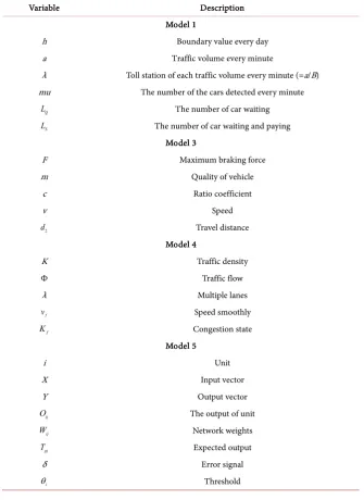
We analysis the electronic toll station. In general, the number of the traffic roads is 2 or 3, L > B, the number of manual toll station must be greater than 1. We assume the number of the toll stations are 3, B = 3. By collecting and han-dling the data, we get the traffic volume per day (h) and minute (a). Then we calculate a/B to the λ, delimiting the λ as the toll station of each traffic volume every minute. By consulting data, we can get mu that is the number of cars tested each minute. We get the Table 3.

Table 2. Traffic volume statistics every day and minute.

Average Daily Traffic Volume Daily Boundary Value (h) Traffic Volume Every Minute (a)

1 - 1500 1500 0.520833333

1501 - 4000 4000 1.388888889

4001 - 10,000 10,000 3.472222222

10,001 - 25,000 25,000 8.680555556

25,001 - 75,000 75,000 26.04166667

DOI: 10.4236/ajor.2018.83013 225 American Journal of Operations Research

Table 3. Some data of only 3 electronic channels.

Average Daily Traffic h a λ (=a/B) mu LQ LS

1 - 1500 1500 0.52 0.17 30 0.00 0.01

1501 - 4000 4000 1.39 0.46 30 0.00 0.02

4001 - 10,000 10,000 3.47 1.16 30 0.00 0.04 10,001 - 25,000 25,000 8.68 2.89 30 0.00 0.10 25,001 - 75,000 75,000 26.04 8.68 30 0.00 0.29 75,001 - 300,000 300,000 104.17 34.72 30 0.08 1.24

From the Table 3, we learn that when B = 3, the maximum traffic volume can be sustained. So, the electronic toll station has 1.24 cars queuing for waiting.

Step 2. Manual toll station’s reference value

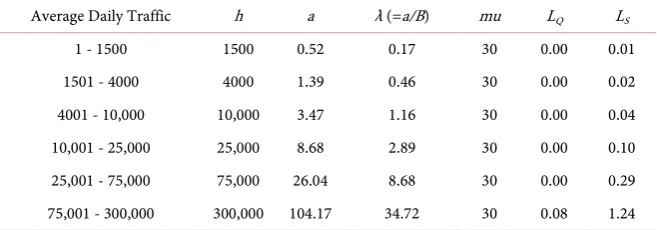
Because the time of manual toll is longer than electronic toll, we choose three sets of data to analysis. See the following of three tables.

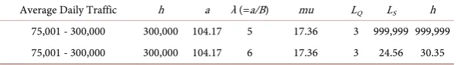
From Table 4, we come into conclusion that when B = 3, the total number of cars reaches 75,000, but the number of waiting cars is too big to come true. So, we add a new toll gate, B = 4, to get Table 5.

When the manual toll station to 4, then the number 25,000 to the 75,000 stag-es was significantly reduced. But the toll station cannot withstand the traffic flow of more than 75,000. Then add 1 or 2 station comparisons, Table 6.

We can know that when the number of manual toll collections is 6, the max-imum traffic volume can be sustained, so we select the reference value of the queuing vehicles for the 30.35 toll stations.

On the whole, we select electronic toll station when the number of queuing vehicles reference value is 0.43; the selection of the number of queuing vehicles at the manual toll station reference value of 10.12.

4. Multiple Weight Model Based on Analytic Hierarchy

Process

We chose the 4 most important factor analysis. According to the symmetry of the freeway in both directions, we choose a direction to study.

4.1. Weight Distribution Based on Analytic Hierarchy Process

These four factors are the cost of the toll booth, the waiting time of the vehicle, the average charging time and the number of traffic accidents. Analytic hie-rarchy process is a combination of quantitative and qualitative analysis of deci-sion-making methods. It is decomposed into various constituent elements through complex problems, and then divided into ordered hierarchical struc-tures according to the dominant relationship of factors [3].

1) The cost of defining electronic toll booths is 5 million, and that of artificial ones is 1 million. The weight is 1.

DOI: 10.4236/ajor.2018.83013 226 American Journal of Operations Research

Table 4. Some data of only 3 manual channels.

Average Daily Traffic h a λ(=a/B) mu LQ LS

1 - 1500 1500 0.52 0.17 3 0.00 0.06

1501 - 4000 4000 1.39 0.46 3 0.00 0.15

4001 - 10,000 10,000 3.47 1.16 3 0.00 0.39 10,001 - 25,000 25,000 8.68 2.89 3 0.04 1.00 25,001 - 75,000 75,000 26.04 8.68 3 24.21 27.10 75,001 - 300,000 300,000 104.17 34.72 3 999,999 999,999

Table 5. Some data of only 4 manual channels.

Average Daily Traffic h a λ (=a/B) mu LQ LS

1 - 1500 1500 0.52 0.13 3 0.00 0.04

1501 - 4000 4000 1.39 0.35 3 0.00 0.12

4001 - 10,000 10,000 3.47 0.87 3 0.00 0.29 10,001 - 25,000 25,000 8.68 2.17 3 0.00 0.72 25,001 - 75,000 75,000 26.04 6.51 3 0.26 2.48 75,001 - 300,000 300,000 104.17 26.04 3 999,999 999,999

Table 6. Some data of 5/6 manual channels.

Average Daily Traffic h a λ (=a/B) mu LQ LS h

75,001 - 300,000 300,000 104.17 5 17.36 3 999,999 999,999 75,001 - 300,000 300,000 104.17 6 17.36 3 24.56 30.35

3) The charging time for the electronic toll booths is defined as 2 seconds and the manual time is 20 seconds. The weight is 2.

4) The number of traffic accidents is average. The weight is 1.

4.2. Standardized Treatment and Selection

We use 75,001 - 30,000 as a reference. The data is shown in Table 7.

Because of the different factor units, the data needs to be normalized before the weighted values, so that the weight of each factor is consistent and compara-ble in the calculation. We use SPSS to normalize data. According to the weight calculation and comparison, the corresponding weights are shown in Table 8.

In the above table, the smaller the weight, the lower the total cost, the shorter the vehicle waiting time, the shorter the payment time, and the fewer traffic ac-cidents, the more reasonable the plan. It was found through observation that when the number of kiosks was 4—2 electronic toll stations and 2 manual toll stations—the weight value was about 0.3. At this time, the construction cost is about 460,000, the average vehicle payment time is 0.46, and the traffic accident is about 0.39, which is the best optimization plan.

5. Braking Distance and Speed Model

DOI: 10.4236/ajor.2018.83013 227 American Journal of Operations Research

Table 7. 5 factors related to the numerical value.

Average Daily

Traffic Terminal Number Electron Number Number Manual Cost Reference Value Charge Time Accidents Traffic

75,001 - 300,000 4

3 1 40 8.5175 6.5 1

2 2 30 15.795 11 1

1 3 20 23.0725 15.5 2

0 4 10 30.35 20 3

5

4 1 42 7.062 5.6 1

3 2 34 12.884 9.2 1

2 3 26 18.706 12.8 2

1 4 18 24.528 16.4 3

0 5 10 30.35 20 3

Table 8. Weight comparison.

Average Daily Traffic

Terminal

Number Electron Number Manual

Toll

Number Cost

Reference

Value Charge Time Accidents Weight Traffic

75,001 - 3,00,000

4

3 1 1.34295 −0.01072 −1.3481 −0.84584 0.48124 2 2 0.46309 0.685 −0.46486 −0.84584 0.30048 1 3 −0.41678 1.38072 0.41838 0.39039 1.35593 0 4 −1.29664 2.07644 1.30161 1.62662 2.41139

5

4 1 1.51892 -0.14986 −1.52475 −0.84584 0.51739 3 2 0.81503 0.40672 −0.81816 −0.84584 0.37278 2 3 0.11114 0.96329 −0.11157 0.39039 1.46439 1 4 −0.59275 1.51987 0.59502 1.62662 2.55601 0 5 −1.29664 2.07644 1.30161 1.62662 2.41139

transportation tools or machinery. It is affected by many factors such as quality, speed, braking force, road, climate and so on [4]. Here we assume that only by the quality, speed and braking force, other factors hardly affect.

In this model, we use the maximum braking force F, which is equal to the change in the vehicle’s kinetic energy, and F is proportional to the vehicle’s mass

m.

In the braking force (F) car driving distance (d2) for Fd2, and the speed from v to 0, the kinetic energy change is mv₂2 , according to the hypothesis.

2

2 mv₂

Fd = . (14)

Because the brake acceleration when a is constant, by Newton’s second law F ma= _{, into 2} 2

2

mv

DOI: 10.4236/ajor.2018.83013 228 American Journal of Operations Research 2

2

d =cv _{. (15)} Through the search results, when the average speed is 80 km/h, and the pro-portion coefficient at this time is c = 0.013. We can know:

(

)

2

2 0.013 80 0 83.6 m

d =cv = × − = _.

So, the braking distance is 83.6 m.

6. Traffic Flow Model

6.1. Model Principle

When studying highways, it is necessary to study the factors related to freeway traffic flow models and the establishment of expressway traffic flow models [5]. In this model, we estimate the results based on speed (v), traffic density (K) and traffic flow (Φ).

Under normal conditions, the freeway is divided into multiple lanes (λ) in a single direction. It is assumed that there is no difference between vehicles and each lane is not affected. Get the equation:

Kv

λ

Φ = . (16) According to real life, when the traffic flow increases, the traffic density be-comes larger and the speed bebe-comes smaller, and vice versa. This shows that there is a certain relationship between speed and density, and the speed is in-versely proportional to the density. Assuming they are decreasing linearly, c0 is a normal value. In addition, as the density increases, the rate of decrease of speed should increase.

0

d d

v _c

K = − . (17)

0

d d

v _{c K}

K = − . (18) When the traffic density is 0, the speed can reach the ideal type, that is, the speed is stable (vf). When traffic density reaches a crowded state (Kf), speed

0

v= .

( )

v v

k

= = = . (19)

( )

v K K

K

= = =

. (20) According to the Formula (18), (19) and (20), we can learn

2

1 , 0

f f

f K

v v K K

K

 _{ } 

 

= −_ _ < <  _{ } 

 

. (21)

Combine (16) and get the new equation.

2 1 f f K v K K

λ     Φ = − _ _

 _{ } 

 

DOI: 10.4236/ajor.2018.83013 229 American Journal of Operations Research Highway traffic flow model is what we get. The model is a response to the re-lationship between speed, traffic flow and density.

6.2. Mapping Relationships

In order to understand the characteristics of the function more intuitively, we use MATLAB to draw the diagramv K− _{. See Figure 1.}

It can be seen that density is inversely proportional to vehicle speed. The speed reaches a maximum of 120 and the traffic density approaches 0; when the speed is 0, we get K=25_.

Then use R to draw the diagramv− Φ. See Figure 2.

It can be seen that when the traffic density reaches 15 or so, the traffic flow reaches a maximum value of 2400; before 15th, the traffic flow is proportional to the increase; after 15th, because of the road congestion problem, the traffic flow decreases inversely and gradually becomes 0.

6.3. Analysis of Different Traffic

Based on the data collected, we assume an average of 2500 vehicles per day

Figure 1. K v− relation graph.

DOI: 10.4236/ajor.2018.83013 230 American Journal of Operations Research during the normal period, with a peak period of 50,000. That is, the normal pe-riod is 104 vehicles per hour, and the peak pepe-riod is 2083 vehicles per hour. Know that:

1)Light period

When the traffic volume is 104 per hour, there are the following two condi-tions.

a) The traffic density is 2 and the speed is almost 120 km/h, smoothly. b) The traffic density is 24 and the speed is almost 20 km/h, crowded. 2) Heavy period

When the traffic volume is 2083 vehicles per hour, the traffic density is 15 and the speed is almost 80 km/h.

7. Fuzzy Neural Network Model Based on BP Algorithm

7.1. Model Principle

Fuzzy neural network is a massively parallel processing network system used to simulate human brain functions. Fuzzy logic is a mathematical method of accu-rately processing uncertain information. It depends on the rules given by the do-main experts [6]. There is no formal framework to select the parameters of the fuzzy system. Neural networks have the advantages of learning ability, self-adaptive ability, and fault tolerance. It can handle complex, non-linear and uncertain problems.

In this case, we use a fuzzy-BP neural network model; the structure diagram is shown in Figure 3.

The general BF algorithm includes two steps: forward and backward propaga-tion. That is, when calculating the error output, we will follow the direction from input to output, and the adjustment weight and threshold will be output to in-put. In forward propagation, the input signal acts on the output node through the hidden layer, and the output signal is generated by a nonlinear transforma-tion [7]. If the actual output is inconsistent with the expected output, the back propagation process shifts to error. Error back propagation is to invert the out-put error to the inout-put layer through the hidden layer and spread the error to all cells of each layer, and the error signal obtained from each layer serves as the ba-sis for adjusting the weight of each cell. By adjusting the connection strength

DOI: 10.4236/ajor.2018.83013 231 American Journal of Operations Research between the input node and the hidden layer node, the connection strength and the thresholds of the hidden layer and the output node, the error decreases along the gradient direction. After repeated learning and training, determine the net-work parameters (weights and thresholds) that correspond to the minimum er-ror and stop training. At this point, the trained neural network can input infor-mation into similar samples, and the processed inforinfor-mation is not linearly transformed with minimal output error.

With n examples of learning samples [8], input vector X =

(

)

expected output vector Y=

(

)

signal is δ. The learning process is as follows:

1) Initializing the weights of the network Wij

( )

θ

( )

2) Input sample set

{

}

3) Transfer function is Sigmoid, output from input to output Opi. Set the unit

element, the output of unit i and of layer K is Opi. The input of the next layer,

section K + 1 and section j, is netpj =

∑

(

)

(

)

(

)

{

}

1 1 exp

pj j pj i ij pi j

ij pi j

O f net f W O

W O θ θ   = = _ − _   = ÷ + _− − _

∑

∑

(

)

1

1 2 1

p pj pi

k p p

E T O

E E

k =

= −

=

∑

∑

4) If E E≤ s (system average error tolerance) or Ep≤Eps (error tolerance

of a single sample) or to the specified number of iterations, the learning is over. Or, error back propagation, turn to E.

5) Calculating the error of each unit of the network layer by layer:

(

)(

)

pj Opj Opj Tpj Opj

δ = − − _{(output layer). (25)}

(

)

pj Opj Opj plWpl

δ = −

∑

6) The correction of each weight and unit threshold is calculated:

(

)

( )

(

)

( )

1 1

ij pj pj ij

j pj j

W n O W n

n n

ηδ α

θ ηδ α θ

∆ + = + ∆

∆ + = + ∆ (27)

7) Fixed network weights and thresholds:

(

)

( )

(

)

(

)

( )

(

)

1 1

1 1

ij ij ij

j j j

W n W n W n

n n n

θ θ θ

+ = + ∆ +

+ = + ∆ +

(28) Finally, turn to 2.

7.2. Performance Prediction Based on Fuzzy-BP Neural Network

DOI: 10.4236/ajor.2018.83013 232 American Journal of Operations Research security. In terms of safety, we mainly consider highway accidents. We use a combination of manual charging system and electronic charging system to achieve flexible and efficient high-speed charging.

Consider the impact of three aspects, respectively, for the flow and flow of the shopping cart. According to the cost data of road transport and toll stations in the United States, the network inputs 3 and outputs 1 set. 15 sets of data, in-cluding 9 sets of normal training data and 3 sets of variable data as test data.

Step 1. We set up a toll station with 2500 daily traffic as an example and build a model with MATLAB. Get Figure 4 and Figure 5.

Figure 4. Sixth training.

DOI: 10.4236/ajor.2018.83013 233 American Journal of Operations Research The bigger the R-squared is, the more obvious the linear relationship is, which is the closest to the real value in the sixth training.

Step 2. We set up a toll station with 50,000 traffic as an example. The same idea as above shows that Figure 6 and Figure 7 are obtained.

Similarly, the graph shows that the neural network is closest to the true value when trained sixteen times.

Our solution is to conduct a series of training in the neural network model. The error of testing and verification is small, and the gap between real events is not large, reflecting the high performance of the program.

Figure 6. Sixteenth training.

DOI: 10.4236/ajor.2018.83013 234 American Journal of Operations Research

8. Safety Performance Model Based on Factor Analysis

Factor analysis is the statistical techniques of common factors extracted from the variable group. Factor analysis can find the hidden representative factor in many variables. A factor of the same nature as variables can reduce the number of va-riables, but also the relationship between the variables of hypothesis test [9].

1 11 1 12 2 13 3 1

2 21 1 22 2 23 3 2

3 31 1 32 2 33 3 3

1 1 2 2 3 3

p p p p p p

p p p p pp p

y x x x x

y x x x x

y x x x x

y x x x x

µ µ µ µ

µ µ µ µ

µ µ µ µ

µ µ µ µ

= + + + +   _{= + + + +}   = + + + +     = + + + +      

. (29)

The factor analysis of electronic toll station is as follows.

(

)

(

)

(

)

(

)

(

)

G1 0.395 PEDS 0.020 ROUTE 0.628 LGT-COND 0.536 WEATHER 0.043 PERSONS

= + − +

+ +

(

)

(

)

(

)

(

)

(

)

G2 0.013 PEDS 0.648 ROUTE 0.025 LGT-COND 0.536 WEATHER 0.043 PERSONS

= + +

+ +

Manual toll collection system:

(

)

(

)

(

)

(

)

(

)

(

)

(

)

(

)

F1 0.409 PERSONS 0.097 PEDS 0.172 ROUTE

0.436 MAN-COLL 0.392 REL-ROAD 0.22 LGT-COND

0.096 WEATHER 0.030 DRUNK-DR

= + − + − + + − + + + −

(

)

(

)

(

)

(

)

(

)

(

)

(

)

(

)

F2 0.124 PERSONS 0.017 PEDS 0.126 ROUTE

0.080 MAN-COLL 0.027 REL-ROAD 0.621 LGT-COND

0.449 WEATHER 0.445 DRUNK-DR

= + +

+ + − +

+ +

From these equations we can learn: (Table 9).

The KMO value is 0.549, which is close to 1; the Bartlett value is 6871.015; and the Sig. is 0 < 0.005. First we know that it has a strong correlation (Table 10).

The table is a matrix of component score coefficients used to calculate the common factor score. Three factors can be obtained, that is, the validity of the road, that is, the values of F1 and F2 mentioned above.

From the factor analysis, it can be concluded that after the increase of driver-less vehicles, traffic accidents caused by human errors are reduced, thereby im-proving safety performance. Under the condition of high-performance electron-ic toll collection system, safety performance is improved and traffelectron-ic accidents are reduced.

Table 9. KMO and Bartlett test.

The Kaiser-Meyer-Olkin measure of sampling sufficiency 0.549

Sricity test of Bartlett

Approximate chi square 6871.015

df 28

DOI: 10.4236/ajor.2018.83013 235 American Journal of Operations Research

Table 10. Component score coefficient matrix.

Ingredients

1 2 3

PERSONS 0.409 0.124 −0.065

PEDS −0.097 0.017 0.787

ROUTE −0.172 0.126 0.034

MAN_COLL 0.436 0.080 −0.191

REL_ROAD −0.392 −0.027 −0.301

LGT_COND 0.022 0.621 0.148

WEATHER 0.096 0.449 −0.009

DRUNK_DR −0.030 0.445 −0.274

Therefore, we should increase the use of electronic charging systems to op-timize the establishment of toll collection stations.

9. Conclusions

According to the best plan and related data, we use CAD drawing software to draw a simple graph, as shown in Figure 8.

Combining the figure, we describe our design in detail from Shape, Size, Merging Pattern and Accident Prevention.

1) Shape

Because the charging time of the electronic toll booths is short, the cars only need to be decelerated instead of parking, so the electronic toll booths can be set mainly; and the grooves just entering the toll plaza (such as the trapezium in

Figure 8) can help the cars slow down and reduce the pressure of the toll pla-za.

2) Size

According to the figure, two electronic toll collection stations are located in-side the toll plaza, close to the opposite lane, and the electronic toll booths are about 1m wide; there are 2 manual toll booths with a width of 2 m. Each vehicle has a width of 3 m and a total of 18 m.

3) Merging Pattern and Accident Prevention

When we choose electronic and artificial combination design, drivers will slow down from the groove to the toll booth, reducing traffic congestion to some extent. When it was discovered that there was no car at the electronic toll booth, the car could also be switched to another toll channel. This design not only makes it possible to reduce the time pressure on the toll plaza, but also facilitates passenger travel.

10. Strengths and Weaknesses

10.1. Strengths

DOI: 10.4236/ajor.2018.83013 236 American Journal of Operations Research

Figure 8. Schematic diagram of one-way toll plaza.

2) Traffic flow: Highway design and operation management play the greatest role.

3) Fuzzy-BF neural network: neural network: with learning ability, self-adaptive ability, fault tolerance and so on. It can handle complex, non-linear and uncertain problems.

10.2. Weaknesses

1) Traffic flow: Unable to solve abnormal and unexpected traffic conditions. 2) Fuzzy-BF neural network: There is a possibility of network training failure, and there is currently no good optimization program.

10.3. Later Optimization

With the increase of driverless vehicles, traffic accidents caused by human errors have decreased and safety performance has improved. In order to adapt to the arrival of unmanned driving, the setting of high-performance electronic toll col-lection system can not only improve the safety performance, reduce traffic acci-dents, but also reduce the charging time and cater to changes in the times. Therefore, we should increase the use of electronic charging systems to optimize the establishment of toll collection stations.

Acknowledgements

This work was supported in part by the Chinese college students’ training pro-gram for innovation and Entrepreneurship under the Grants CJ17017 and D17027. The effective suggestions provided by the article have been approved by the relevant organizations.

References

[1] American Embassy in China (2016) An Overview of the Current Status of American Freeway Charges. http://blog.sina.com.cn/s/blog_67f297b00102wo16.html

[2] Mo, Z., Yu, J. and Sun, Y. (2003) Poisson Distribution Based Mathematic Model of Producing Vehicles in Microscopic Traffic Simulator. Journal of Wuhan University of Technology, No. 1, 73-75.

DOI: 10.4236/ajor.2018.83013 237 American Journal of Operations Research Weights with Analytic History Process. Henan Science, No. 8, 1140-1144.

[4] Kim, J.G., Kwon, S.T., Yoon, S.C., et al. (2011) Infrared Thermographic Analysis of Railway Brake Disc during Braking. Key Engineering Materials, 488-489, 597-600. [5] Chen J.Q., Qian W. and Zhang, C. (2017) Research on Model Optimization Design

of Expressway Toll Station. Journal of Times, No. 20.

[6] Jiang, S.F. and Zhang, S. (2008) Damage Identification Method of Data Fusion Structure Based on Fuzzy Neural Network. Engineering Mechanics, 25, 95-101. [7] Yu, J., Zhang, J., Wu, J. and Wang, X. (2015) Evaluation and Strategic Research on

Sustainable Supply of Important Mineral Resources. Economic Daily Press, St. Thomas.

[8] Liu, N., Yang, Y. and Zhao, Y.M. (2009) Evaluation of Teaching Quality with Fuzzy-BP Neural Network. Journal of Sichuan University of Science & Engineering, No. 3, 29-31.