Comparisons of VAR Model and Models Created by
Genetic Programming in Consumer Price Index
Prediction in Vietnam
Pham Van Khanh
Military Technical Academy, Hanoi, Vietnam Email: [email protected]
Received May 30,2012; revised June 30, 2012; accepted July 10,2012
ABSTRACT
In this paper, we present an application of Genetic Programming (GP) to Vietnamese CPI inflation one-step prediction problem. This is a new approach in building a good forecasting model, and then applying inflation forecasts in Vietnam in current stage. The study introduces the within-sample and the out-of-samples one-step-ahead forecast errors which have positive correlation and approximate to a linear function with positive slope in prediction models by GP. We also build Vector Autoregression (VAR) model to forecast CPI in quaterly data and compare with the models created by GP. The experimental results show that the Genetic Programming can produce the prediction models having better accuracy than Vector Autoregression models. We have no relavant variables (m2, ex) of monthly data in the VAR model, so no prediction results exist to compare with models created by GP and we just forecast CPI basing on models of GP with previous data of CPI.
Keywords: Vector Autoregression; Genetic Programming; CPI Inflation; Forecast
1. Introduction
Inflation has great importance to saving decisions, in- vestment, interest rate, production and consumption. De- cisions basing on impractical inflation predictions result in uneffective resource allocation and weaker macroeco- nomic activities. Meanwhile, better predictions see better forecast solutions given by economic agents and improve the entire economic performance.
Different models depending on the theory of different price fixation are often used for describing inflation evo- lutions. These models emphasize the role of different variables in inflation. The different econometric models have different modeling specification, and information quality. Despite of huge explained variables in models basing on theory to improve the level of conformity, they uncertainly ameliorate the ability of prediction models.
One can see many different models in different coun- tries, particularly: the model of Phillips curve with added expecting elements, traditionally monetary model, price equations basing on monetary demand viewpoint.
Apart from theoretic inflation ones above, it can be seen the variable time series models which are used for inflation data in the past so as to forecast further inflation and give no more explaination to analyze. Recently, the multivariate time series model and its variations have
appeared in nonlinear time string, especially in the smooth transition regression. Nevertheless, with the con- tent of the paper, we just present models relevant to this study without deeply analyzing their theoretic base.
2. Methodology
We center on considering the VAR model and applica- tions of Genetic Programming to forecast the inflation index CPI. Initially, estimate and accreditation to be good models, and then predictions will be seen based on variables taken from models.
2.1. Vector Autoregression Model
The vector autoregression (VAR) model is one of the most successful, flexible, and easy way to use models for the analysis of multivariate time series [1].
Before 1980s, equation models were simultaneously used for analyzing and forecasting macro-economic vari- ables as well as the study of the economic cycle. At that time, econometric were dedicated to issue of the format of the model-relating to properties of endogenous vari- ables in the model.
nomic theory or visual knowledge of model, determin- ing the presence or absence of the variables in each equa- tion.
Sim [2] has changed the concerns of contemporary economist community. He said that most of the economic variables, especially macroeconomic variables are en- dogenous. On the other hands, they are interactive. There- fore, he proposed a multivariable model with endogenous variables having the same role. Nowadays, the VAR model has become a powerful tool and was used exten-sively (especially in macro-economic problems), predic-tions (particularly the medium-term and long-term ones), and the analysis of shock transmission mechanism (con-sidering the impact of a shock on a dependent variable on other dependent variables in the system).
When presenting the VAR model, one can introduce it structurally and then contractionally. Nonetheless, for the prediction, we can use the information from the resulting estimates of the shortened model, so it is better to solely present the contracted model serving to experimental analysis without the detail structure model to avoid un- necessary complexities.
A basic VAR contraction forms:
1 1 0
t t p t p t
y A y A y B x Bq t qx CDtut
, , Kt
y y y
, , Mt
x x x
D
where t 1t is a K-dimension endogenous
variable observed, t 1t is a M-dimension
exogenous variable observed, t concludes the ob-
served deterministic variables such as the constant, linear trend, the fake crop as well as the other user-defined
white noise, is the process of K-dimensional 0 ma-
trix, and plus determines socks expecta-
tion covariance.
t u
t t
uE u u
, ,
j j A B C
0, ,
p p
matrixes are the appropriate number of dimensions on themselves.
Although our purpose just forecasts, we also men- tioned somewhat another important application of VAR model—the analysis of the shock transmission mecha- nism, reaction function and variance disintergration. How- ever, calculating the reaction functions and variance dis-intergrations need parametric estimates in structural VAR models, we have unnecessary deeply interest in these problems but only conduct experimental analysis.
However, as mentioned in the introduction, another application of the VAR model is the analysis of shock transmission mechanism being done by reaction function and variance disintergration. We should not delve into analyzing the structural VAR model although calculating the reaction functions and variance disintergrations need parametric estimates in the model.
We use the VAR model for Vietnam’s inflation fore- casts because of its effective predictions, so general building and estimating VAR models will be introduced. Sample is the first concern before estimating the model. A large sample gives us vacant orders to estimate, and
better estimate accuracy. However, with time series, the large sample (overlong string) raises issues about the stability of estimate coefficients in the model. Even in the countries with political and economic stability, policy changes in internal economy, and external action vary the relation of economic variables. Hence, monthly data is the best choice because of its sufficient free orders and stablility in the system. Usually, no monthly data exist to a macro variable, and then industrial production values used.
The parameters in VAR model are estimated following steps:
1) Testing the stationary of data series. If the data se- ries non-stationary, we will check integrated community relations. If the relation occurs, VECM switched.
2) Lag Length Selection:The lag length for the VAR(p)
model maybe determined using model selection criteria. The general approach is to fit VAR(p) models with orders
max
and choose the value of p which mini-
mizes some model selection criteria. The three most common information criteria are the Akaike information criterion (AIC), Hannan-Quinn criterion (HQC), Schwarz information criterion (SIC), etc.
Latency optimizations are chosen by minimizing the following standard information:
2 2 2 * * 2AIC log det ,
2 log log
HQ log det ,
2log
SC log det ,
FPE det ,
u
u u
K u
n n nK
T T
n n nK
T T
n n nK
T T n n n T n
where u n
is estimated by T1
Tt1uˆ ˆtut, n is thenumber of parameters in every equation. Maybe, differ- ent standards are shown by different models. Hence, models with the most effective forecast are to be contin- ued.
3) Diagnosing and simplifying the model.
Checking the stability of the model statistically. If
roots of the model are greater than or equal to 1, the model is nonstationary.
Residual test: testing for autocorrelation of residual and testing for heteroskedasticity.
Simplifying the model: Estimate results of the model
(after being well-tested) provide statistical informa- tion about the role of lagged variables in the equation. Therefore, we will use these informations to verify if some lagged variables are statistically significant or not, so we should or should not remove any lagged variables of model.
Analyzing and forecasting after having an effective model.
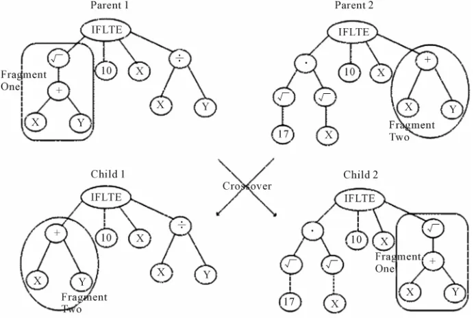
change between parents. Its operators include the follow- ing steps:
Selecting randomly in each parent one node.
2.2. Genetic Programming Swapping their positions.
The crossover operator is shown in Figure 1.
Mutation: Mutation is the process of variation of a
chromosome set created. The process includes the fol- lowing steps:
Genetic Programming (GP) is an automatic learning method thought from biological evolution with the target of establishing a computer program to meet the learners’ expectation, so the GP is one of machine learning tech- niques using evolutionary algorithms to optimize com- puter programs following the compatibility of a program to calculate. The GP had tested since the 1980s, but until 1992, with the born of the book “Genetic Programming: On the Programming of Computers by Means of Natural Selection” by John Koza [3], it was visibly shaped. How- ever, in the 1990s, the GP just solved simple problems. Today, together with the development of the hardware as well as the theory in the first half of 2000, the GP has grown rapidly.
Choosing a node on the parent.
Canceling the seedling on the node chosen.
Birthing accidentally a new seedling on above posi-
tion.
2.2.1. Primary Handling Steps for the GP
Existing five significant steps for primary handling the GP that a programmer need to establish:
1) Setting leaf nodes (such as independent variables, nonparametric functions, aleatory constants) for each branch of the evolution programming.
Chromosome: Chromosome (a term borrowed from
biological concepts), as in biology, determine the good level of an individual. The GP evolves a computer pro- gram representing under tree-like structure. The tree is easily evaluated by a recursive procedure. Each node on the tree is a calculating function, and each leaf stands for a class math, using for simple evolutionary and estimable mathematical expressions. As usual, the PG is an expres- sion of the tree-like procedure.
2) Collecting evolutional functions for each branch of evolution programming.
3) Pointing out a good fitness (measuring the compa- tibility of each individual in a population).
4) Determing parently the parameters controlling opera- tion (individual volume, chromosome amount, variation probability ···).
5) Defining the criterion for finishing or the method for determining the result of the running process.
Operators in the GP: Crossover and Mutation are
two main operators used in the GP. These are also two terms borrowed biology, and two main factors affecting to evolution process.
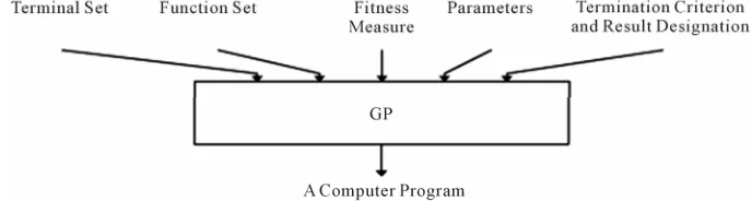
The diagram above (Figure 2) shows that if a GP is
considered a “black box” with the input hold the primary handling steps, after going through the GP, the result received is a computer program (function to forecast).
[image:3.595.125.471.489.721.2]Crossover: Shows the process of chromosome ex-
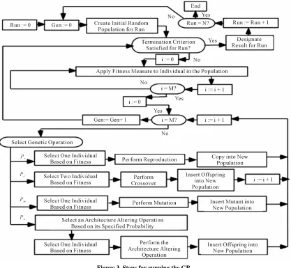
Figure 2. Primary handling steps for the GP.
2.2.2. Steps for Running the GP
A typical GP starts running with an accidental program made up by possible elements. Then, the sequential GP changes the population through many generations by using the operator in the GP. The selection process equates to count each individual property. An individual chosen to join in gene problems or canceled depends on its property (the way to value property given in the 3rd
preparing step). The loop transformation of populations is the main content and is repeated many times in a program of GP. The sequence with the changeable po- pulation is the main sequential content in the GP.
Steps for running the GP is shown in Figure 3 and
includes the following steps:
1) Initializing incidentally a population (zero gene- ration) with individuals created by functions, and leaf nodes.
2) Repeating (generations) follow postauxiliary until the condition satisfied.
3) Operating individuals to determine their property. 4) Choosing 1 or 2 individuals from the population with probability depending on their property to parti- cipate in the Gene problems in step 3).
5) Creating new individuals to the population by applying the post gene problems with specified proba- bility.
6) Reproducing, and copying the selection into new
populations.
7) Crossover: creating subindividual by combining se- quentially portions of them.
8) Mutation: creating subindividual by replacing a new portion of the individual into its old one.
9) Structural changes: Being done by changing the structure of the individual selected. After satisfying the condition of last criterion the operation of the best in- dividual means that the result of running process is ex- posed, and we receive the solution for problems basing on an effective operation of the individual.
2.2.3. Application of Genetic Programming (GP) to Prediction Problem
This section presents the method of applying GP for pre- diction/forecasting problems. The detail description can be found in a number of previous publication [4-6]. The
task of time series prediction is to estimate the value of the series in the future based on its values in the past. There are two models of time series prediction: one-step prediction and multi-step prediction. In one-step predic- tion, the task is to express the value of y t
n
as a func- tion of previous values of the time series, y t
1 ,
,y tn
and other attributes. That is to find the func-
tion F so at: th
1
1 1
1 , , ; 1 , ,
; ; k 1 , , k k
y t F y t y t n x t
x t p x t x t p
1 , ,
y t y t n
where
1 , ,
1
1
are the values of the time
series in the past and x t1 x tp
1
are the values of x attributes in the past and
1 , ,
k k k
x t x tp are the values of xk attributes
in the past. This equation is based on an assumption that the value of the time series y depends on its previous values and also the values of some other attributes in the past. Fore xample, for CPI inflation prediction, the value of CPI in the future may depend on its previous values and thevalues of some other factors like total domestic product (GDP), monetary supply (M2), and soon. The purpose of multi-step prediction is to obtain predictions of several steps ahead into the future, y t
, 1 ,y t
2 ,
y t
1 t
starting from the information at current time slice . In this paper, we only focus on one-step prediction/forecasting.
3. Empirical Results
3.1. Description of DataThe data used in the model was provided by the General Statistics Office (GSO). We took information from two following data set to forecast.
Quarterly data: Over the period of 2nd quarter of 1996
to 4th quarter of 2011, monthly data: from January 1995
to February 2012. The data by 4th quarter of 2010 or De-
Figure 3. Steps for running the GP.
(0.115) (0.108)
[0.000] [0.000]
{ 5.685} { 5.176}
(0.156) (0.101) [0.008] [0.001] { 1.749} { 3.369}
ˆ
0.651 1 0 2 1 0.559 2
0.272 3 0.304 3
str p t gex t
gex t gm t gex t
gcpi t gex t
monthly data. Variables in the model are described in
Table 1.
3.2. Estimating Inflation Forecast Models
3.2.1. The VAR Model for Inflation Predictions
3.2.1.1. Modeling Experimental Estimates
From steps for raising and estimating the model, we re- ceive the VAR model with just 3 variables such as gcpi, gex and gm2 through all tests. The last model audited as:
} ) ˆ
1
42 gcpi t
gcpi t
6] }
3 gcpi t
(0.132) (0.357) (0.127) [0.106] [0.052] [0.021] { 2.418} {1.947} { 2.229 (0.128) (0.358) (0.136 [0.103] [0.005] [0.07 { 1.629} {2.779}
0.319 1 0.696 2 1 0.291
0.208 2 0.994 2 2 0.2
str p t
gex t gm t
gex t gm t
{ 1.774
(2)
(0.039) (0.109) (0.118) [0.051] [0.000] [0.000] {1.951} { 10.057} { 6.442}
(0.050) (0.099) [0.027] [0.005] { 2.005} { 2.828}
ˆ 2
0.076 1 1.092 2 1 0.762 2 2
0.109 3 0.2800 2 3
str p t gm t
gex t gm t gm t
gcpi t gm t
(1)
Table 1. The name of variables in used model.
Variable name Signs Growth
Total domestic product with the price in 1994 gdp ggdp
Consumer price index compared to the
previous month cpi gcpi
The US dollar price index compared to
previous month Ex Gex
Commodity import turnover im gim
Monetary supply M2 Gm2
The model met the demand of stability, autocorrelation, changeable error variance tests. In fact,
Modeling stability checking.
After estimating the VAR model, we need to test its stability. The test determines whether roots of character- istic polynomial belong to unit circle or not. All roots in
Table 2 are less than 1 in module. Therefore, the VAR is
acceptable thanks to stable equation.
Table 2: Checking the stability of the model through
roots of typical polynomials by endogenous variables:
gcpi4, gex4, gm2.
Test for the autocorrelations of residuals.
Results of Portmanteau Tests basing on Q test (Table 3)
showed that with lagged steps, p in Q test is greater than
5%. This means hypothesis H0 not to be canceled (no
residual autocorrelations).
Testing for Heteroskedasticity.
The residual Heteroskedasticity tests are carried by general tests about heteroskedasticity of White. The re- sult of White test showed that no heteroskedasticity re- mains. The result is introduced in Table 4.
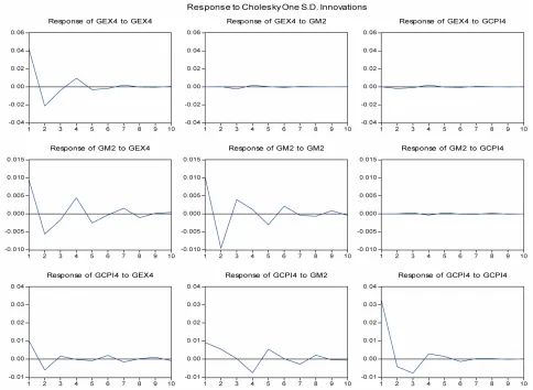
Impulse Response Functions.
With the model estimated, we can analyze the shock transmission mechanism through response functions. To recieve the response function, some constraints are ap- plied for the equation. Constraints chosen are Cholesky Disintegrate ones. The Cholesky used serially: gex, gcpi.
Choosing the order depends on inflation changes without effects on exchange rate. Analyzing performance is as in
Figure 4.
The first two figures see inflation changes struggled by the shock itself, which is descending and being vanished for a 5 quarter. Monetary supply and exchange rate shock influences seems to impact insensibly on Vietnam’s in- flation.
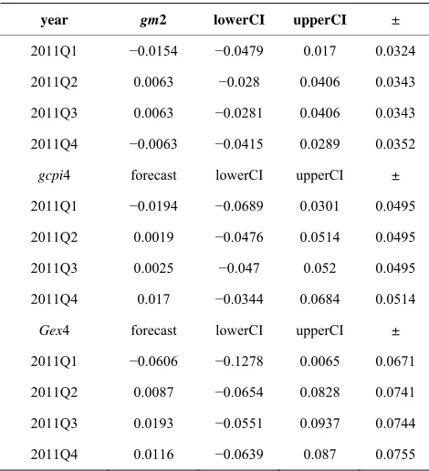
3.2.1.2. Prediction Results 1) Inflation predictions for 2011
For inflation predictions in 2011, we use the models (1)-(3) to estimate and data by 2010 to apply the model and make forecasting procedures for 2011. Acquired re- sults are given in the following Table 5.
Table 2. Unit root test.
Root Modulus
−0.316094 − 0.767403i 0.829954
−0.316094 + 0.767403i 0.829954
0.010726 − 0.758628i 0.758704
0.010726 + 0.758628i 0.758704
−0.712593 − 0.062363i 0.715317
−0.712593 + 0.062363i 0.715317
0.276312 − 0.618574i 0.677482
0.276312 + 0.618574i 0.677482
−0.461363 0.461363
No root lies outside the unit circle.
VAR satisfies the stability condition.
Table 3. Tests for autocorrelations of residuals.
VAR Residual Portmanteau Tests for Autocorrelations
Null Hypothesis: no residual autocorrelations up to lag h
Lags Q-Stat Prob. Adj Q-Stat Prob. df
1 3.318091 NA* 3.374330 NA* NA*
2 5.494490 NA* 5.625777 NA* NA*
3 7.178825 NA* 7.398761 NA* NA*
4 13.37463 0.1464 14.03713 0.1210 9
5 25.29735 0.1169 27.04373 0.0782 18
6 27.95866 0.4131 30.00074 0.3141 27
7 36.30709 0.4543 39.45180 0.3183 36
8 39.24429 0.7135 42.84087 0.5638 45
9 42.83282 0.8630 47.06266 0.7368 54
10 47.15679 0.9319 52.25144 0.8309 63
11 58.41922 0.8760 66.04216 0.6754 72
12 65.36161 0.8970 74.72015 0.6751 81
*The test is valid only for lags larger than the VAR lag order df is degrees of
freedom for (approximate) chi-square distribution.
Table 4. Results of white test.
VAR Residual Heteroskedasticity Tests: Includes Cross Terms
Joint test:
Chi-sq df Prob.
322.3132 324 0.5160
S
Figure 4. Response function-shock transmission mechanism. The Table 2 sees the increase of inflation gcpi, ex-
change rate and monetary demand, but it is hard to com- pare with real inflation to value its property. In doing so, we do a counter-process of considering the inflation in- crease in comparison with real inflation. The result given in Table 6.
See the table above, it’s obvious that square roots of average square prediction errors is 1.38. The grestest quarterly variance is 3%, pointing out that the acquired model is quite effective.
2) Inflation predictions for 2012
For inflation predictions in 2012, we use the model (1)-(3) to estimate and data by 2011 to apply the model and make forecasting procedures for 2012. Acquired results are given in Table 7.
3.2.2. Applications of the GP for Inflation Predictions
3.2.2.1. GP Parameters Settings
To tackle a problem with GP, several factors need to be clarified beforehand. These factors often depend on the problem and the experience of the system user (practi- tioner). The first and important factor is the fitness func-
tion. Traditionally, for symbolic regression problems, the
fitness function is the sum of the absolute (or some times the square) error. Formally, the (minimising) fitness function of an individual is defined as:
1 Fitness = n i i
i
y f
y
where N is the number of data samples (fitness cases), i is the value of the CPI in the data sample, and fi is
the function value of the individual at the point in
the sample set (
th i fi is the fitted value of i).
To assess the consistency of a model created by the GP, we put additional quantities:
y
1 Test Fitness = N i i
i n
y f
, 1, ,
y i n N
where i
, 1, , y i n N
, 1, ,
y i n N
is real value of CPI in the test
data sample ( for monthly data i is real
value of CPI from 2011M1 to 2012M2, for quaterly data
i
f y
is real value of CPI from 2011Q1 to
2011Q4), and i is the predicted value of i. Some
Table 5. Prediction results of gcpi from model for 2011.
year gm2 lowerCI upperCI ±
2011Q1 −0.0154 −0.0479 0.017 0.0324
2011Q2 0.0063 −0.028 0.0406 0.0343
2011Q3 0.0063 −0.0281 0.0406 0.0343
2011Q4 −0.0063 −0.0415 0.0289 0.0352
gcpi4 forecast lowerCI upperCI ±
2011Q1 −0.0194 −0.0689 0.0301 0.0495
2011Q2 0.0019 −0.0476 0.0514 0.0495
2011Q3 0.0025 −0.047 0.052 0.0495
2011Q4 0.017 −0.0344 0.0684 0.0514
Gex4 forecast lowerCI upperCI ±
2011Q1 −0.0606 −0.1278 0.0065 0.0671
2011Q2 0.0087 −0.0654 0.0828 0.0741
2011Q3 0.0193 −0.0551 0.0937 0.0744
2011Q4 0.0116 −0.0639 0.087 0.0755
Source: Estimates of author. The prediction result witnesses some 95% accuracy, lower confidence interval, upper confidence interval and just vari- ances in last column.
Table 6. Comparisons the forecast results and actual infla- tion for the CPI in 2011.
CPI(real) CPI(predict) Prediction error square errorPrediction
2011Q1 102.1700 100.0016 −0.0212 0.00045
2011Q2 101.0900 102.3641 0.0126 0.00016
2011Q3 100.8200 101.3427 0.0052 0.00003
2011Q4 101.3700 102.5339 0.0115 0.00013
Square root of prediction mean square error 0.013856558
Source: Estimates of author.
where
0 if
0
my log , mysinsh
ln if 0 2 ,
x x e e
x
x x
x x
1
0my log is , mysqrt
1 x
x x
e
if 0 , if 0
x
x x
0 if 0if 0 x
x
mydivide ,y x y
x
3.2.2.2. Applying Quarterly Data for Forecasting
On the basis of selected variables from the VAR model,
Table 7. Results for predicting gcpi in the model for 2012.
Prediction of gcpi
forecast lowerci upperci ±
Prediction of cpi
2012q1 −0.0146 −0.0788 0.0496 0.0642 99.88999
2012q2 0.0224 −0.0441 0.0888 0.0665 102.1275
2012q3 0.0363 −0.0325 0.1051 0.0688 105.8348
2012q4 −0.006 −0.0795 0.0674 0.0735 105.1998
[image:8.595.308.536.103.205.2]Source: The forecast results for the directly acquired growth rate from pre-dicting model for CPI are contributed to prediction performance in the model and 4th quarterly of 2011.
Table 8. Run and evolutionary parameter values.
Parameter Value
Population size 250
Generations 40
Selection Tournament
Tournament size 3
Crossover probability 0.9
Mutation probability 0.05
Initial Max depth 6
Max depth 30
Max depth of mutation tree 5
Non-terminals mylogis, mysqrt, mydivide, sin, cos.+, −, /, −, exp, mylog, mysinsh, Terminals cpi(t− 1), ···, cpi(t− 12), ex(t− 1), ···,
ex(t− 4), gm2(t− 1), ···, gm2(t− 4)
Raw fitness mean absolute error on all cases fitness
Trials per treatment 50 independent runs for each value
we have established models for inflation predictions. Nevertheless, favorable models witness the dependence of CPI on its values in the past.
Prediction model (a)
4 ( 2)3 4 4
ˆ 4
1
cpi t
cpi t cpi t cpi t
cpi t cpi t
cpi t
e
(4)
where cpi tˆ
is the prediction of cpi t
. Acquired re-sults of predictions for 2011 using model (a) are given in the following Table 9.
It can be seen that square roots of average square pre- diction errors is 0.45%, and 0.9% means the grestest quarterly variance. The predictions for 2012 and 2013 are given in Table 10.
[image:8.595.308.537.261.520.2] [image:8.595.61.286.427.533.2]
2 2
ˆ 1 sin ( 1) sin sin ( 1) sin ( 1)
1
( 2) ( 3)
1 exp exp sin sin sin
( 4)
1
( 2) ( 1) cos
1 exp ( 1) ( 1)
cpi t cpi t cpi t cpi t cpi t f
f
cpi t cpi t
g cpi t
g cpi t cpi t
cpi t cpi t
( 4) cpi t (5)
The formula (7) below employing data by 2011 shows go
Acquired results of predictions for 2011 using model
(b) are given in the following Table 11. od performance:
Evidently, square roots of average square prediction errors is 0.55%, and 1.1% means the grestest quarterly variance.
The predictions for 2012 and 2013 using model (b) are given in Table 12.
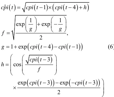
Prediction model (c)
ˆ 1 4
1
3
cpi t cpi t cpi t h
cpi t 1 1 exp exp , 2
1 exp 4
3 cos
exp 3 exp
2
g g
f
g cpi t cpi t
cpi t h f cpi t (6)
[image:9.595.120.388.106.202.2]The sequence of model (6) is as ineffective as that of model (5). The result is not introduced here.
Table 9. Predictions for 2011 using the data by 2010.
Time Real data Prediction Prediction error square errorPrediction
2011Q1 102.17 101.341 0.0081146 0.0000658
2011Q2 101.09 101.236 −0.0014416 0.0000021
2011Q3 100.82 101.228 −0.0040451 0.0000164
2011Q4 101.37 101.406 −0.0003582 0.0000001
Square root of prediction mean square error 0.0045939
Table 10. Predictions for 2012, 2013 using the data by 2010.
2012 2013
Time Q1 Q2 Q3 Q4 Q1 Q2 Q3 Q4
Forcast 101.72 101.40 101.13 101.27 101.48 101.43 101.28 101.28
1 sin 4 3 cos 3 44 1 2
1 sin
1 3
cpi t
f
cpi t cpi t
f
g cpi t cpi t
cpi t cpi t cpi t
g cpi t
cpi t cpi t (7) The predictions for 2012 and 2013 using this for ar
on Monthly Data
future based
ˆ 1
cpi t cpi t
mula e given in Table 13.
3.2.2.3. Forecasts Basing
Here, we have predicted CPI values in the
[image:9.595.311.539.239.354.2]on its previous ones. Data from January 1995 to December
Table 11. Predictions for 2011 using the data by 2010.
Time Real data Prediction Prediction error square error Prediction
2011Q1 102.17 101.15 0.0100748 0.0001015
2011Q2 101.09 101.31 −0.0021692 4.705E-06
2011Q3 100.82 1
e ro di u
01.18033 −0.0035268 1.244E-05
2011Q4 101.37 101.31303 0.0005635 3.176E-07
Squar ot of pre ction mean sq are error 0.0054535
data by . Table 12. Predictions for 2012, 2013 using the 2010
2012 2013
Ti em Q1 Q2 Q3 Q4 Q1 Q2 Q3 Q4
Forecast 101.37 101.05 100.82 101.19 01.21 01.02 00.8 1 1 1 2 101.10
Table 13. Predictions for 2012, 2013 using the data by 2011.
2012 2013
Ti e Q1m Q2 Q3 Q4 Q1 Q2 Q3 Q4
[image:9.595.97.286.318.479.2] [image:9.595.310.537.460.572.2] [image:9.595.58.285.541.653.2]T . P ns e of e- cember 2012 us
Time M 7 M8 M9 M1 M12
20 t t ise m el, e r t tim f
January 2011 to February 2012 are used for testing. S
11are aken o ra the od thos ove he e o
imilary, The reference of prediction accuracy relies on data in March and April 2012.
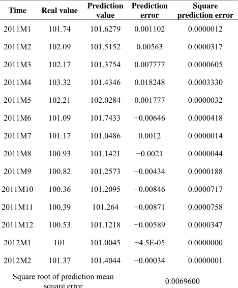
We introduce some models found out by GP with the min fitness (98.0298) for CPI predictions:
ˆ 11 5 1 2 12
10
cpi t cpi t cpi t cpi t
sin 7 8
2 sin 9 7
sin cpi t cpi t
cpi t cpi t cpi t
e
(8) In Table 14, we see that the greatest monthly error is
1.83%. Square roots of average square prediction erro are 0.00696 which is much less than predictions of V
102.0122, real data 100.05 and error 1.961 ar
3.
nce of prediction models created
10.
value error prediction error
1
rs the AR model.
Inflation forecasts in March 2012 is 101.697, but ac- tual data are 100.16, and error 1.535%. Similarly, infla- tion forecasts
e in April 2012. March data took one-step prediction, and then two-step prediction for April ones, means that using March data predicts following month.
Prediction results over the time of May to December 2012 in below Table 15.
[image:10.595.57.291.449.732.2]2.2.4. Evaluating the Consistence of the GP For evaluating the consiste
Table 14. Predictions using the data by 20
Time Real value Prediction Prediction Square
2011M1 101.74 101.6279 0.001102 0.0000012
2
−
root dictio
squ r .0069
011M2 102.09 101.5152 0.00563 0.0000317
2011M3 102.17 101.3754 0.007777 0.0000605
2011M4 103.32 101.4346 0.018248 0.0003330
2011M5 102.21 102.0284 0.001777 0.0000032
2011M6 101.09 101.7433 −0.00646 0.0000418
2011M7 101.17 101.0486 0.0012 0.0000014
2011M8 100.93 101.1421 −0.0021 0.0000044
2011M9 100.82 101.2573 0.00434 0.0000188
2011M10 100.36 101.2095 −0.00846 0.0000717
2011M11 100.39 101.264 −0.00871 0.0000758
2011M12 100.53 101.1218 −0.00589 0.0000347
2012M1 101 101.0045 −4.5E-05 0.0000000
2012M2 101.37 101.4044 −0.00034 0.0000001
Square of pre
are erro
n mean 0 600
able 15 redictio
ing the data b results ov
y 2010.
r the time May to D
5 M6 M 0 M11
Forecast 101.8 101.5 101.29 101.15 101.04 100.96 100.99 101.073
b , c e l e q rl d
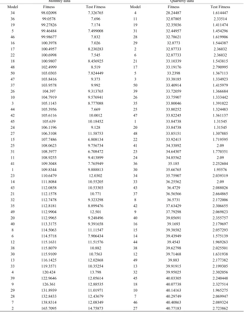
side and outside sample. A model fitting to both past y GP we onsid r 50 mode s to very uarte y an monthly forecasts, and examine the relation of errors in
and future data (on the other hands, the error inside sam- ple is small, that of outside sample also similar) is called the consistent model. Prediction models of the GP would be considered to be consistent if small fitness implied small test fitness, meaning that test fitness is a varied flow function of the fitness.
We received following equation thanks to carrying out test fitness linear regression basing on quarterly models:
Test Fitness 0.053016 Fitness
2
Std.Error 0.001453 0.226003, 1.319782
R DW
(9)
The correlation coefficient between test fitness and fitness is 0.485. Therefore, it can be valued tha
prediction models are consistent because of regressive re
5
t quarterly
sults (9), and positive correlation equation between the test fitness and the fitness.
Similarly, monthly data have regressive model as: Test Fitness 0.087980 Fitness
Std.Error 0.00168
2 0.520951, 1.905514
R DW
(10)
The data for regressive models (9) and (10) from Table A in Appendix A. The correlati
between test fitness and fitness is 0.751, therefore, from re
e VAR model for inflation prediction has suc- ceeded in selecting fitting models in line with currently e take predictions for 2011 from the are getting on coefficient
gressive result (10), with positive lope and positive correlation between test fitness and fitness, it can be seen that monthly prediction models of GP are consistent. Additionally, monthly models witness a bigger correla- tion between test fitness and fitness against quarterly ones.
4. Conclusions
Using th
available data. If w
VAR model to be comparision standard, square roots of average square prediction errors is 1.38. The best im- pressive error by months is not greater than 3%. Using the model to forecast for 2011 with accuracy 95% indi- cates that inflation in the 1st quarter of 2012 decreases
slightly, it continuously witnesses somewhat increase in the 2nd and the 3rd quarters. The performance needs test-
and state expense, and prolong inflation lead to hi
itself di
s funded by The Vietnam nce and Technology Deve- Above results from the VAR model show that recently
have been resulted from different causes, especially un- controlled stimulus packages, uneffective public invest- ment
gh inflation rate in economy. This confirms how im- portant the application of monetary policies with a con- sistent attitude for improving the credibility of policies is. Consistence when applying monetary policies is also one way to impact on inflation expectation we desire.
Errors of prediction results from models created by the GP are much less than those of the VAR model. One benefit from using the GP to raise the prediction model is that we don’t need to specify the model (the GP
scovered the model), and propose hypothesizes for variables in the model. GP can provide some analytical formulas for prediction of the model so the GP is called “white box”, unlike the neural network model called “black box”, which shows us the predicted value, without giving analytical expressions. Analytical expressions also help us to detect relationships between variables in fore- casting models and assess interactions between them. GP can also help us to detect relationships between eco- nomic variables that economic theory can not detect or exceed human judgments. So the greatest advantage of GP comes from the ability to address problems for which there are no human experts. Although human expertise should be used when it is available, it often proves less than adequacy for automating problem-solving routines. Nonetheless, the GP can’t indicate the accuracy of pre- diction values and their distribution. Moreover, predic- tion functions for the GP are often complicated, and dif- ficult to explain. That’s all about disadvantages of the GP. These show that the CPI in the future just depends on its values currently and previously but other variables. Ob- viously, Vietnam’s inflation rate mainly bases on its citi-
zens’ expectation, particularly in the late of December 2011, salary increases for evil servants released by gov-
ernment and applied from 1st May 2012 has followed
price augment from January 2012 without basing on other elements.
5. Acknowledgements
The work in this paper wa National Foundation for Scie
lopment (NAFOSTED), under grant number 10103- 2010.06.
REFERENCES
[1] J. Hamilton, “ Princeton Univer-
sity Press, Prin
80, pp. 1-48.
s, Cambridge,
al Time Series Prediction,” Proceedings of Euro
recast with Anticipation Using Genetic Pro- Time Series Analysis,”
ceton, 1994.
[2] C. A. Sims, “Macroeconomics and Reality,” Economet- rica, 1980, Vol. 48, No. 1, 19
[3] J. Koza, “Genetic Programming: On the Programming of Computers by Natural Selection,” MIT Pres
1992.
[4] M. Santini and A. Tettamanzi, “Genetic Programming for financi
Genetic Programming, Lake Como, 18-20 April 2001, pp. 361-370.
[5] D. Rivero, J. R. Rabunal, J. Dorado and A. Pazos, “Time Series Fo
gramming,” 8th International Work-Conference on Artifi- cial Neural Networks, Computational Intelligence and Bio- inspired Systems, Barcelona, 8-10 June 2005, pp. 968-975. [6] J. Li, Z. Shi and X. Li, “Genetic Programming with
Wavelet-Based Indicators for Financial Forecasting,” Tran- sactions of the Institute of Measurement and Control, Vol. 28, No. 3, 2006, pp. 285-297.
Appendix A: Fitness and Test Fitness Results 50 Models Created by GP
Table A. Fitness and test fitness results 50 models created by GP is ascending sorted by fitness value.
Monthly data Quarterly data
Model Fitness Test Fitness Model Fitness Test Fitness
34 98.02098 7.326765 4 28.24487 1.614447
36 99.0578 7.696 11 32.07805 2.33514
19 99.27826 7.174 19 32.35036 1.411474
5 99.46484 7.499008 31 32.44957 1.454296
46 99.98677 7.832 28 32.78621 1.619906
16 100.3978 7.026 29 32.8773 1.544387
17 100.4957 8.230283 2 32.87733 2.36032
22 100.6998 7.545 6 32.87733 2.36032
18 100.9807 8.456925 21 33.10339 1.543815
48 102.4999 8.519 17 33.19176 2.790995
50 103.0303 7.824449 5 33.2398 1.367113
47 103.8416 9.373 3 33.38185 1.334923
37 103.9578 9.992 50 33.40914 1.415979
26 104.397 9.313765 39 33.72059 1.366684
10 104.7919 9.576941 26 33.75907 1.333442
3 105.1143 8.777088 35 33.80046 1.391022
44 105.3956 7.669 25 33.80252 1.324483
42 105.6116 10.0012 47 33.82245 1.361137
45 105.639 10.18452 1 33.84738 1.31545
24 106.1196 9.128 20 33.84738 1.31545
27 106.3108 11.58753 48 33.85151 1.307885
15 107.7486 6.808134 22 33.92415 1.719595
25 108.0623 9.756734 41 34.33892 2.09
31 108.3977 6.708472 23 34.64307 1.770351
11 108.9255 9.413899 24 34.85562 2.09
41 109.3048 7.765949 36 35.185 2.252604
1 109.8344 9.888813 30 35.66765 1.95576
23 110.6479 12.0302 34 35.75907 2.039319
14 111.8084 10.55205 33 36.25562 2.09
43 112.0858 10.53303 43 36.4729 2.088026
21 112.1578 10.771 37 36.56566 2.664865
32 112.7478 9.323298 8 36.5731 2.172006
35 112.8181 8.899476 42 37.63429 2.306655
49 112.9904 12.501 9 37.79298 2.069823
20 112.9965 9.248496 40 39.05691 2.355757
40 113.3175 9.391658 16 39.1693 2.179697
8 114.5063 11.11547 15 39.38582 2.057293 6 114.5718 7.906434 14 39.43949 1.575139
12 115.1631 11.51576 44 39.4543 1.969263
38 115.8079 10.882 38 39.62798 2.025501
30 115.9109 10.7563 12 39.71468 1.631938
13 116.1425 12.02868 49 39.883 2.177382
33 119.3571 10.35254 13 39.91915 2.199305
4 120.424 13.798 32 39.95025 2.302056
39 122.9646 12.05614 45 40.03305 2.240448
9 126.361 12.88535 18 40.07738 2.327514
29 131.8939 11.01971 10 40.14163 1.965275
28 132.8433 12.43679 7 40.29749 2.069947
Appendix B: Some Prediction Function Created by GP with Small Fitness and Test Fitness
(Monthly Data)
Model 34
sin 7 81
ˆ 5 1 11 2 12
10
sin 9 7 sin cpi t cpi t
cpi t cpi t cpi t cpi t c
f cpi t cpi t e
2
pi t f
Fitness = 98.02098, Test Fitness = 7.326765
Model 36
myl og(mylogis( ( -9)))
1ˆ 3 12 6 4 1 10 2
10
mysqrt 3 cpi t 9 6 4
cpi t cpi t cpi t cpi t cpi t cpi t
cpi t e cpi t cpi t cpi t
cpi t
9
Fitness = 99.0578, Test Fitness = 7.696
Model 19
1
ˆ 4 1 2 2 7 2
10
cpi t
cpi t cpi t cpi t cpi t 9
3cpi t
12
Fitness = 99.27826, Test Fitness = 7.174
Model 5
1
ˆ 5 1 sin 2 3 2 7
10
cpi t
cpi t cpi t cpi t cpi t 2cpi t
12
Fitness = 99.46484, Test Fitness = 7.499008
Model 31
1
ˆ 1 my log 12 mysqrt 10
10
3 my log mysqrt my log 12
cpi t cpi t cpi t cpi t
cpi t cpi t
1
6 cpi t
cpi t
Fitness = 108.3977, Test Fitness = 6.708472
Appendix C: Some Prediction Function Created by GP with Small Fitness and Test Fitness
(Quaterly Data)
Model 4
ˆ 1 4 cos 4
2 4
cos 1 4 cos my log is
2 5
2 1 2 2
my log is cos
2 2
cpi t cpi t cpi t f cpi t
m t m2 t 5
f cpi t cpi t
m t
m t m t
g
m t
g
Fitness = 28.24487, Test Fitness = 1.614447
Model 11
2 2 2 3
ˆ 1 mydivide ,
2 3
2 3 2 4 2
mydivide my sinh my log ,
2 4
m t m t
cpi t cpi t f
m t
m t m t m t
f
m t m
1 2 2
2 2
m t
t
Fitness = 32.07805, Test Fitness = 2.33514
Model 48
ˆ 1 4 my log mysqrt my log
cpi t cpi t cpi t cpi t2
Fitness = 33.85151, Test Fitness = 1.307885
Model 19
ˆ 4 1
my log my log is 4 my log is 4 4
my log is 1 my log is 3 my log is 4
cpi t cpi t cpi t f
f cpi t cpi t cpi t
g cpi t cpi t cpi t
4
g
cpi t
Fitness = 32.35036, Test Fitness = 1.411474
Model 20
ˆ 1 4 m
cpi t cpi t cpi t y log is cpi t1