Localization of a Single Sensor with Respect to a Single Beacon using Received Signal Strength (RSS) in Terrestrial Environment

Localization of a Single Sensor with Respect to a Single

Beacon using Received Signal Strength (RSS) in

Terrestrial Environment

Anisur Rahman

Dhaka, Bangladesh

Shafayet Khan

Dhaka, Bangladesh

Khalid Bin Salahuddin

Dhaka, Bangladesh

ABSTRACT

This paper apprised the issue of finding the location of a single sensor node with a single beacon in a terrestrial wireless sensor network (WSN). Generally, the localization of a single sensor node in a terrestrial sensor network can be solved using multilateration technique with respect to three or more known beacon nodes. However, there is an area of concern, when the localization of a single sensor node (i.e. mobile station, cell phone) is to be measured with respect to only one known beacon node i.e. base transceiver station (BTS). Such a challenge is aimed to be solved with the help of received signal strength (RSS) survey data for a particular location within the desired environment. A simulated terrain and a model has been created based on RSS Survey data that defines the contours of radio frequency (RF) coverage in a particular test facility under a single beacon node. Simulation results show that our proposed model gives a solution which converges to determine the location of a single sensor node with respect to a single beacon node.

General Terms

Localization Algorithms

Keywords

Wireless Sensor Networks, Received Signal Strength, Localization, Single Beacon, Heat map

1.

INTRODUCTION

This document undertook the research subject knowing well the fact that, the growing population of mobile devices and bandwidth-hungry applications; mobile network traffic is set to explode in the near future. Industry research predicts that aggregate wireless traffic will increase by 1000 times within the next decade [1]. Positioning in wireless networks is today mainly used for yellow page services. Yet, its importance will grow when emergency call services become mandatory as well as with the advent of more advanced location-based services. It is also plausible that future resource management algorithms may rely on position estimation and prediction [2]. We talked briefly about the wireless sensor network (WSN) technology and about its significance in wireless communications and advances and how localization can be of use in this particular field. Moreover, we presented a general concept for base transceiver station (BTS) and its use in a global system for mobile communication (GSM) network.

Localization has widely been explored in terrestrial wireless sensor network and various mechanisms have been proposed. Generally these methods can be classified into two categories: range-based and range-free schemes. The former apply inter node distances to multilateration or triangulation whereas the latter rely on profiling. Being applicable for almost every scenario, mobile localization based on cellular network has

gained increasing interest in recent years. Since received signal strength (RSS) information is available in all mobile phones, RSS-based techniques have become the preferred method for GSM localization. Although the GSM standard allows for a mobile phone to receive RSS information from up to seven base stations (BSs), most of the mobile phones only use the information of the associated cell (i.e. BS) as its estimated position. Therefore, the accuracy of GSM localization is seriously limited [3].

WSNs are a significant technology attracting considerable research interest. Recent advances in wireless communications and electronics have enabled the development of low-cost, low-power and multi-functional sensors that are small in size and communicate in short distances. Cheap, smart sensors, networked through wireless links and deployed in large numbers, provide unprecedented opportunities for monitoring and controlling homes, cities, and the environment. In addition, networked sensors have a broad spectrum of applications in the defense areas, generating new capabilities for reconnaissance and surveillance as well as other tactical applications [4].

As mobile devices spring up and with the corresponding improvements of wireless communication, localization in mobile networks has become one of the hottest topics in wireless and mobile computing research [5, 6]. However, it is a key problem to acquire sufficient localization accuracy for location-based services (LBSs).

A broad spectrum of solutions, such as RSS, time of arrival (TOA) [7], time difference of arrival (TDOA) [8], and angle of arrival (AOA) [9], has been proposed to attain mobile localization by measuring the radio signal traveling between a mobile terminal and base stations [10, 11]. Some researchers have proposed a number of methods including fingerprinting and max-min box [12]. These techniques, except for RSS, often depend on additional hardware, which means additional cost.

Although the global positioning system (GPS) [13] is considered to be the most well-known localization technique, it is not available in many cell phones, requires direct line of sight to the satellites, and consumes a lot of energy. However, WiFi chips, similar to GPS, are not available in many cell phones, and not all cities in the world contain sufficient WiFi coverage to obtain ubiquitous localization.

networks (WLANs), but they would appear to be attractive also for wireless sensor networks.

In [19], Elnahrawy et al. proposed several area-based localization algorithms using RSS profiling; these algorithms are area based because instead of estimating the exact location of the non-anchor node, they simply estimate a possible area that should contain it. Two different performance parameters apply: accuracy, or the likelihood that an object is within the area, and precision, i.e., the size of the area.

2.

PROBLEM DOMAIN

Problem domain and the environmental constraints surrounding the problem begin with a detailed outlay of the problem and the environmental constraints.

In a wireless network, many issues can arise which can prevent the radio frequency (RF) signal from reaching all parts of the facility. Examples of RF issues include multipath distortion, fading, hidden node problems and proximity issues. A site survey helps define the contours of RF coverage in a particular facility. It helps to discover regions where multipath distortion can occur, areas where RF interference is high and find solutions to eliminate such issues. A proper site survey provides detailed information that addresses coverage, interference sources, equipment placement, power considerations and wiring requirements. The site survey documentation serves as a guide of network design [20].

A solitary traditional BTS can only find the possible quadrant of a sensor node when they establish a link with that BTS. Our problem scenario arises for an area under the coverage of a solitary BTS where the mobile station (MS) wants to know its probable two-dimensional location within the BTS’s coverage area. Usually, in city and urban area there are multiple BTSs which can perform localization using one of AOA, triangulation or multilateration method.

The case resumes with a worse case situation with the possibility of or combination of such reasons as in geographical, political, economic or technological drawbacks where a certain area happens to have a solitary BTS with a specific credible range. There is a question of interest as to how a solitary BTS is going to perform localization in such a scenario. The answer to this question is that a solitary BTS can only find out the quadrant position in which the MS resides. However, this paper would show that the location of a particular MS can be figured with more precision within a particular quadrant with our proposed method. A BTS can have 1 to 16 cell sectors. Generally, it possess up to 3 or 4 cell sectors operating under four different directional antennae. Each cell sectors covers an area with a wedge shaped area with each having the same angular span for the same BTS.

The test BTS’s coverage area has been divided into four cell sectors (quadrants) where each quadrant spans exactly by 90 degrees. In order to find a narrowed down location of a MS within the coverage area of this already established problem scenario which has a distinctive terrain, we are going to consider the coordinate values of the area along the XY surface for simplicity. Moreover the RSS Survey data were collected beforehand to find the respective RSS reading of each separate squared grid on the two-dimensional XY coverage surface.

2.1

Environmental Constraints

For our proposed method, the size of the area we have worked with is a 2 × 2 km area and was represented with a digital elevation model with the resolution of 100 m. Even for such a

small area, this should produce a total of 400 grids (considering there were no grids where surveillance could not be performed because of natural or artificial hindrance). These grids should be deterministically, as well as manually explored at certain positions within each grid and their corresponding RSS readings received by the exploring mobile unit should be acknowledged and recorded as per each grid. It can be assumed that the calculated signal level at each 100 ×100 m is very close to real situation. However, for a hilly terrain, a terrain with forestry or a lake, it would quite difficult to arrive at every grid positions per 100 m for RSS checking due to lack of flat or solid ground.

With the RSS data and output power of base station, it would be possible to estimate the distance between the mobile

device and BS using Friis transmission equation. The problem is that the distance is calculated using the RSS reading.

In propagation, signal sometimes suffer interference and shadow fading, and the distance calculated would not

always be the exact distance between the BS and the MS and so cannot be considered always for localization calculations. However, for areas with distorted RSS data, different techniques need to be taken into consideration to determine the close to perfect distance reading.

The main idea is to make good use of the cell information, to locate a two-dimensional position and minimize the influence of disturbance, barriers, or non-line-of-sight (NLOS) errors, for example, on performance.

2.2

RSS Profiling

Firstly a predictive approach should be followed. A model of the RF environment should be created using tools. It is essential that correct information on the proposed environment is entered in the RF modeling tool, including location and RF characteristics of barriers like walls or large objects.

To make sure that correct information on the environment were entered in the RF modeling tool in the first place, a passive approach should be followed soon after, where a site survey application should be deployed in the problem field which passively listens to WLAN traffic to detect access points, measure signal strength and noise level.

Steps to perform the aforesaid tasks are detailed below:

 Create an environment diagram in order to identify potential radio frequency obstacles within the surveyed RF environment.

 Manually inspect the environment to look for potential barriers (hills or mountains) or the propagation of radio frequency signals and identify metal rocks and places like lakes or rivers.

 Identify access points that are highly used and the once that are not used.

 Determine preliminary access points (APs) locations.  Make sure to use the same AP model for the survey that

is used in production. While the survey is performed, relocate APs as needed and re-test them once more.  Document the findings. Record all the individual

locations (two-dimensional) and log of all the signal readings (RSSs).

3.

SIMULATION OF TEST TERRAIN

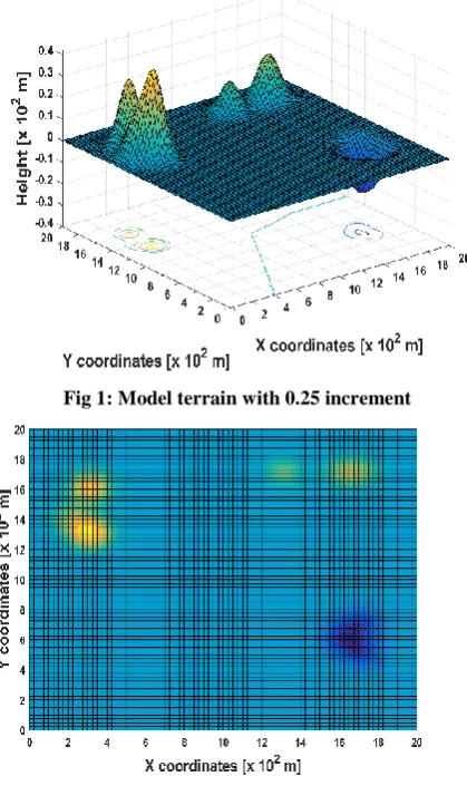
Matlab R2016a has been used for coding and implementing the simulation of a 20×20 meshgrid terrain as displayed in Figure 1. We built environmental Peaks and Pits on our model surface over certain grids. This was done to create individual impressions for hilly, forestry and lake like element that could be present under any BTS. Although, we were not able to draw a BTS within the proposed terrain, but the surface’s (X,Y,Z) = (0,0,0) coordinate should be imagined as the point where the BTS is actually located. A reminder to the readers here is that this is not the whole terrain that would be under the coverage of a solitary BTS. However, this terrain represents only a certain area of one of the four quadrants that was divided by the 4 directional antenna used in cell sectoring with a 90° span each.

Fig 1: Model terrain with 0.25 increment

Fig 2: Model terrain (top view)

In Figure 1, the 20 × 20 meshgrid defined has an increment of 0.25 ( 102 _{) from 0 ( 10}2 _{) to 20 ( 10}2 _{). A total of six} peaks and three pits were simulated over the terrain using the surfc function. A function named peak provided the necessary logic for building the peaks and the pits at specific locations within the meshgrid. The coloring of the grids were done based on the height of the terrain with the yellow portions having the highest possible heights and the blue portion representing the lowest ones in terms of height.

Figure 2, gives a top view of the meshgrid, that have been explained in details a while ago, with an increment of 0.25 ( 102 _{) from 0 ( 10}2 _{) to 20 ( 10}2 _{). However, if we} consider this as the basis for RSS Survey, there is a massive total of 6400 grids within the simulated terrain.

Fig 3: Model terrain with 1.0 increment

Fig 4: Model terrain (top view)

In Figure 3, the meshgrid defined has an increment of 1 ( 102 _{) from 0 ( 10}2 _{) to 20 ( 10}2 _{). As a result of this,} less number of grids were produced. To be precise, there are 400 grids in total. Later in Figure 4, a top view image of this meshgrid with an increment of 1 ( 102 _{) from 0 ( 10}2 _{) to} 20 ( 102 _{) was plotted.}

Figure 1 and 2 were created for better visualization and understanding of the test Terrain. On the other hand, Figure 3 and 4 were created in accordance with the RSS Heatmap for our proposed method, with an increment of 1 ( 102 _).

4.

HEATMAP CONSTRUCTION

Friis transmission equation has been defined below:

(1)

Here, is RSS by the mobile station, is TSS from the BTS.

(2)

Here, is the distance between BTS and mobile station and is signal frequency of the BTS, c is the speed of light in vacuum and is the wavelength of the transmitted signal by the BTS.

FSPL formula has been defined and further simplified below:

(3)

Here, in (3), the unit of distance is measured in meters (m) and the signal frequency in hertz ( ).

(4)

Here, in (4), the unit of distance is measured in kilometers (km) and the signal frequency in gigahertz (GHz).

Combining both (1) and (4), we get the following equation:

(5)

Thus, we used a combination of (1) along with (5) for the buildup to our RSS HeatMap. Logics behind the terrain heat map on the basis of RSS survey are mainly to maintain the logical spread of values along the surface using (1) along with the help of (5). Here, the diagonal grids go furthest in terms of maintaining better signal strengths than surrounding grids signal strengths because of the presence of a main lobe in the radiation pattern.

In a radio antenna's radiation pattern, the main lobe is the lobe containing the maximum power. This is the lobe that exhibits the strongest field of strength. In the directional antenna in which the objective is to emit the radio waves in one direction, the lobe in that direction is designed to have higher field of strength than the others on a graph. The surrounding grids in front of the hilly (top left distorted field in the simulated terrain) areas, feet of mountainous areas covering grids sometimes have better signal strengths than usual because of multipath propagation when signals from opposite directions collide with each other with the same phase value and vice-versa.

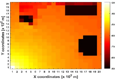
Moreover, the grids those are behind the mountains are being deprived of their usual signal mark because of NLOS errors. Hence we would see a big drop in the RSS values over those grids. Same rationalization was being implemented around and over the forestry areas (top right distorted field in the simulated terrain). Around the pits (impression of a Lake – bottom right distorted field in the simulated terrain) the presence of water on the grids means signal propagation will not be smooth and that signals will be more or less absorbed by water which is why the grids are given very low signal strength values as well as the surrounding grids which are also constantly getting affected from the wayward reflection and multipath propagation of the signal because of the lake.

Fig 5: RSS heatmap of the terrain

Considering all of these factors mentioned above, we created our HeatMap based on RSS readings for a 20 × 20 meshgrid space with a total of 400 grids as shown in Figure 5.

5.

COORDINATES

COMPUTATION

AND

ANALYSIS

Our proposed method works in two simple steps:

 A predetermined RSS HeatMap phase  A real-time tracking phase

During the predetermined phase, a probabilistic RSS HeatMap is constructed, where the RSS from the solitary cell tower at given locations in the area of interest is estimated. The purpose of this predetermined phase is to construct the RSS HeatMap for the solitary cell tower (i.e. BTS) at each location in the fingerprint area. Typically, this requires the surveyor to stand at each location in the fingerprint for a certain period of time to collect enough samples to construct the RSS HeatMap. However, this will increase the fingerprint construction overhead significantly.

During the real-time tracking phase, the RSS HeatMap is used to calculate the most probable fingerprint location at which the user might be standing at that instance. If the real-time tracking phase discovers a single grid as a probable fingerprint location of the user, it tells the user 2D positional information about user’s whereabouts. Otherwise, the person is advised to continue moving in a straight line in any specific direction, for a finite amount of time, for another probable fingerprint location data. This approach strives to determine the possible cluster within the RSS HeatMap where the user might be by eliminating areas of no interest.

Table 1. RSS readings from different sensors positions

Sensor Position Received Signal Strength (RSS)

1

2

3

-52.64 dB

-54.64 dB

-55.67 dB

To simulate the proposed method we have taken into consideration the following scenario as mentioned in the table above. However, a single dataset can contain a minimum of one to finite different positions for the sensor node (i.e. MS) which when needed should be moved in a straight line to aid for the localization calculation. To calculate the coordinates of the actual sensor positions in terms of the grid they are placed at, we need the inter distances between the different positions of the sensor node and their corresponding positions from the beacon node.

The inter distances between the different sensor positions as it moved along a straight line can be calculated from the average walking speed of a human, also taking into consideration, the time it took for the MS to move from one position to the next position. For this particular problem, we have taken a value of 2.82 unit as the inter-position distance between the three sensor positions for simplicity. As per research, the preferred walking speed at which a human choose or tend to walk is about 1.4m/s [21-23]. We have considered the form of 1.4m/s as the preferred walking speed for the user availing our localization technique.

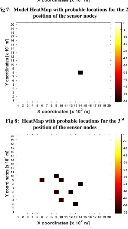
Initially, a RSS HeatMap was plotted based on the probable locations of the first position of the sensor node considering the returned RSS data, as in Table 1, sent from the MS to the BTS. Similarly, respective RSS HeatMaps were plotted based on the RSS data sent from the second and third position of the sensor node. All these have been shown graphically from Figure 6-9 including a combined RSS HeatMap for all the three positions of the sensor node.

Fig 6: HeatMap with probable locations for the 1st position of the sensor nodes

Fig 7: Model HeatMap with probable locations for the 2nd position of the sensor nodes

Fig 8: HeatMap with probable locations for the 3rd position of the sensor nodes

Fig 9: HeatMap with all probable locations for all 3 positions of the sensor nodes

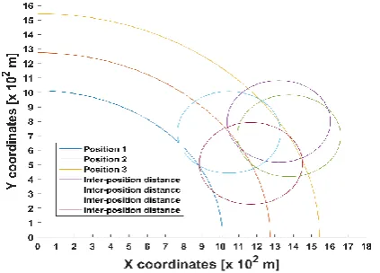
Fig 10: Region covered by 3 positions of the sensor nodes

Fig 11: Narrowed down regions covered by 3 positions of the sensor nodes

In Figure 10, the blue arc was drawn using the distance between the BTS and the first position of the sensor node calculated from (4) using the RSS reading returned by the sensor node at that instance. The red arc was drawn using the distance between the BTS and the second position of the sensor node calculated from (4) using the RSS reading returned by the sensor node at that instance. However, the yellow arc was drawn using the distance between the BTS and the mid-point of the solitary grid representing the third position of the sensor node for more accurate precision. Figure 11 was drawn combining the RSS HeatMap from Figure 9 and the arc graph from Figure 11. This graph further provides more precise ranges for each separate positions of the sensor node.

Fig 12: Region covered by 3 positions of the sensor nodes

Fig 13: Region covered by 3 positions of the sensor nodes

In Figure 12, the track back method was initiated using the distance between the second position and the third position of the sensor node. Two separate circles were drawn using the inter-positional distance of 2.82 units as mentioned previously from the lower and the upper bounds of the third position of the sensor.

In Figure 13, two more separate circles were drawn compared to Figure 12 using the inter-positional distance of 2.82 units as mentioned previously from the lower and the upper bounds of the second position of the sensor.

Fig 14: More narrowed down region covered by 3 positions of the sensor nodes

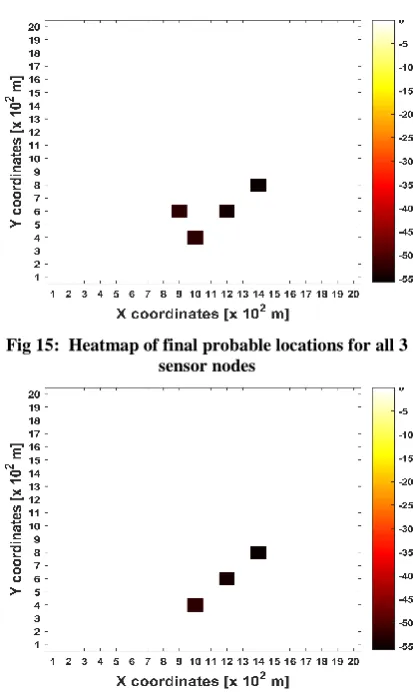
In Figure 14, a graph was drawn accumulating all information gathered from Figure 11-13. This graph further narrowed down the ranges for each projected grid positions of the sensor node. Figure 15 makes use of both Figure 9 and Figure 14 for precise predicted grid localization.

Fig 15: Heatmap of final probable locations for all 3 sensor nodes

Fig 16: Final HeatMap for all 3 predicted grids for all sensor nodes

6.

CONCLUSIONS

In this paper, a method has been successfully implemented on a simulated terrain to determine the two-dimensional location of a single sensor node with respect to a single beacon node using RSS HeatMap. The data for the created RSS HeatMap were generated using pure theory. However, a proper RSS HeatMap should be made considering both the theoretical data and the real-world recorded data. This would produce a far better RSS HeatMap than the one that has been taken to work within this paper. For our proposed method, a 100 area is considered under each grid. However, if the area under each grid is reduced any further, far better accuracy could be achieved but such a policy would be more cumbersome for carrying out any physical RSS survey. There would be an increase in computation complexity as well. Moreover, due to resource limitation while creating the simulated terrain based on theory; numerous other environmental elements are left out to consider. Furthermore, simulation and performance analysis is done on only specific terrain and developed the proposed model around it; however localization in more challenging terrains is also possible with our proposed method.

In future work, clustering algorithms will be considered to reduce the computational complexities that are present in this time in the proposed method.

7.

REFERENCES

[1] Qualcomm Inc., \The 1000x data challenge," [Online] Available: https://www.qualcomm.com/1000x, 2014

[2] Fredrik Gustafsson and Fredrik Gunnarsson, “Mobile Positioning using wireless Networks: Possibility and fundamental limitation based on available wireless networks measurements”, proceedings of the IEEE vol. 22 issue 4, July 2005, PP 41-53.

[3] Huiyu Liu, Yunzhou Zhang, Xiaolin Su, Xintong Li, and Ning Xu, “Mobile Localization Based on Received Signal Strength and Pearson’s Correlation Coefficient”, Hindawi Publishing Corporation, International Journal of Distributed Sensor Networks, Volume 2015, Article ID 157046, 10 pages.

[4] C. –Y. Chong, S. Kumar, “Sensor Networks: Evolution, Opportunities, and Challenges”, proceedings of the IEEE 91 (8) (2003) 1247-1256.

[5] M. Anisetti, C. A. Ardagna, V. Bellandi, E. Damiani, and S. Reale, “Map-based location and tracking in multipath outdoor mobile networks,” IEEE Transactions on Wireless Communications, vol. 10, no. 3, pp. 814–824, 2011.

[6] K. Yu, I. Sharp, and Y. J. Guo, Ground-Based Wireless Positioning, John Wiley & Sons, 2009.

[7] J. Shen, A. F. Molisch, and J. Salmi, “Accurate passive location estimation using TOA measurements,” IEEE Transactions on Wireless Communications, vol. 11, no. 6, pp. 2182–2192, 2012.

[8] J. Saloranta and G. Abreu, “Solving the fast moving vehicle localization problem via TDOA algorithms,” in Proceedings of the 8th Workshop on Positioning Navigation and Communication (WPNC ’11), pp. 127– 130, IEEE, Dresden, Germany, April 2011.

[9] M. Dakkak, A. Nakib, B. Daachi, P. Siarry, and J. Lemoine, “Indoor localization method based on RTT and AOA using coordinates clustering,” Computer Networks, vol. 55, no. 8, pp. 1794–1803, 2011

[10] C. Gentile, N. Alsindi, R. Raulefs et al., “Multipath and NLOS mitigation algorithms,” in Geolocation Techniques, pp. 59–97, Springer, NewYork, NY,USA, 2013.

[11] M. Ibrahim and M. Youssef, “CellSense: an accurate energyefficient GSM positioning system,” IEEE Transactions on Vehicular Technology, vol. 61, no. 1, pp. 286–296, 2012.

[12] M. Bshara, U. Orguner, F. Gustafsson, and L. Van Biesen, “Fingerprinting localization in wireless networks based on received signal- strength measurements: a case study on WiMAX networks,” IEEE Transactions on Vehicular Technology, vol. 59, no. 1, pp. 283–294, 2010.

[13] P. Enge and P. Misra, “Special issue on GPS: The global positioning system,” Proc. IEEE, vol. 87, no. 1, pp. 3–15, Jan. 1999.

[14] P. Bahl, V. Padmanabhan, RADAR: an in-building RF-based user location and tracking system, in IEEE INFOCOM, vol. 2, 2000, pp. 775-784.

IEEE International Symposium on Personal, Indoor and Mobile Radio Communications, vol. 2, 2002, pp. 720-724.

[16]P. Krishnan, A. Krishnakumar, W.-H. Ju, C. Mallows, S. Gamt, A system for LEASE: location estimation assisted by stationary emitters for indoor RF wireless networks, in: IEEE INFOCOM, vol. 2, 2004, pp. 1001-1011.

[17]Teemu Roos , Petri Myllymäki , Henry Tirri, A Statistical Modeling Approach to Location Estimation, IEEE Transactions on Mobile Computing, v.1 n.1, p.59-69, January 2002 [doi>10.1109/TMC.2002.1011059]

[18]S. Ray, W. Lai, I. Paschalidis, Deployment optimization of sensornet-based stochastic location-detection systems, in: IEEE INFOCOM 2005, vol. 4, 2005, pp. 2279-2289.

[19] E. Elnahrawy, X. Li, R. Martin, The limits of localization using signal strength: a comparative study,

in: First Annual IEEE Conference on Sensor and Ad-hoc Communications and Networks, 2004, pp. 406-414.

[20] Http://www.cisco.com/c/en/us/support/docs/wireless- mobility/wireless-lan-wlan/68666-wireless-site-survey-faq.html

[21] Browning, R. C., Baker, E. A., Herron, J. A. and Kram, R. (2006). "Effects of obesity and sex on the energetic cost and preferred speed of walking". Journal of Applied Physiology. 100 (2): 390–398.

[22] Betty J. Mohler, William B. Thompson, Sarah H. Creem-Regehr, Herbert L. Pick Jr, William H. Warren Jr, (2007). "Visual flow influences gait transition speed and preferred walking speed". Experimental Brain Research. 181 (2): 221–228.