Consensus-based Hierachical Demand Side
Management in Microgrid
Jie Ma, Xiandong Ma
Engineering Department, Lancaster University Lancaster, United Kingdom
j.ma6@lancaster. ac.uk, [email protected]
Abstract—The increasing penetration of renewable power generators has brought a great challenge to develop an appropriate energy dispatch scheme in a microgrid system. This paper presents a hierarchical energy management scheme by integrating renewable energy forecast results and distributed consensus algorithm. A multiple aggregated prediction algorithm (MAPA) is implemented based on satellite weather forecast data to obtain a short-term local solar radiance forecast curve, which outperforms the multiple linear regression model. A distributed consensus algorithm is then incorporated into the HVAC (heating ventilation air conditioning) units as the adjustable loads in order to dynamically regulate power consumption of each HVAC unit, based on solar power forecast in a day. The scheme aims to alleviate the local supply-demand power mismatch by varying demand response of the HVAC units. Two case studies are performed to demonstrate the feasibility and robustness of the algorithms.
Keywords-MAPA (multiple aggregated prediction algorithm), hierarchical energy management structure, distributed consensus algorithm, HVAC (heating ventilation air conditioning), microgrid
I. INTRODUCTION
The distributed energy resources have played a vital role in mitigating the pressure of the utility at the peak time. Green energy generation can effectively reduce environmental pollution and hence carbon emissions. Microgrid, as an innovative concept, has been proposed for decades with the aims of compositing distributed energy resources, energy storage device and on-site load demand as a sub-system that in turn can be integrated into the main grid. However, there are many challenges in microgrid, such as diversity of the loads, intermittency and uncontrollability of power generation and load demand. In order to balance power mismatch between local generation and demand, many energy management schemes either in electrical supply side or in demand side in terms of control algorithm implementation have been developed to improve energy dispatch in a standalone microgrid.
A number of literatures have reviewed various approaches to address supply-demand mismatch and power sharing problem. Among them, conventional droop control is the most popular strategy to share active and reactive power among distributed generators in an islanded microgrid, without communication connection [1], [2]. Whereas, in a complex microgrid system, an advanced droop control method is employed to enhance the dynamics of power and frequency [3], [4]. However, it is hard to deal with reactive power sharing when the loads are nonlinear
and unbalanced. Thus, a hierarchical control strategy is presented to consider the economic dispatch problem, in order to improve efficiency, reliability and controllability. The primary and advanced level of the droop control can be implemented in the lower level of hierarchical control architecture, whereas tertiary control can be achieved in the top level [5], [6]. Tertiary control aims at optimizing the operation status of the microgrid based on economic dispatching law, market signal and forecasting results. Multi-agent system (MAS) has been widely used to coordinate the operation of microgrid components under any kind of communication topology. Many researchers have focused on homogeneous devices, such as battery energy storage systems, to eliminate power imbalance with the distributed consensus algorithm [7], [8], where the local power mismatch and battery efficiency can be optimized simultaneously. In the meantime, heterogeneous energy storage devices are considered in [9] along with a cooperative MAS-based control scheme to improve active power sharing. Aggregated controllable loads, as the alternative energy storage devices, can be employed to compensate power mismatch with demand response [10], [11]. Heating, ventilation, air conditioning (HVAC) units, as an indispensable device in the buildings, have been identified to stabilize power mismatch [12]–[14]. However, the existing researches mostly discussed the dynamics of the algorithm under constant power mismatch. In this paper, we will combine a daily renewable power generation with the distributed algorithm to develop an effective load sharing strategy among the aggregated HVAC devices.
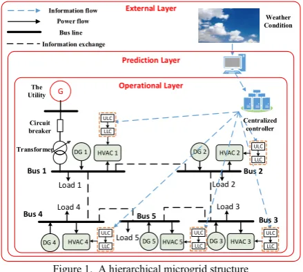
This paper proposes a hierarchical demand side management scheme for the microgrid system. The HVAC device has a good flexibility to overcome time-varying power generation by regulating energy consumption by itself. Furthermore, a MAS framework is introduced to aggregate the homogeneous loads to achieve energy management target. As shown in Fig 1, the proposed hierarchical structure consists of an operational layer, a prediction layer and an external layer. The external layer is responsible for data acquisition. The intelligent forecasting algorithms such as machine learning algorithms and statistic techniques can be employed in the prediction layer [15], [16]. The operational layer aims to investigate economic dispatching strategy. The centralized controller implements the control scheme and provides the operating frequency reference signal to each HVAC’s local controller, which is composed of an ULC (upper layer controller) and a LLC (lower layer controller) to track the reference signal. In this paper, statistical methods including multiple linear regression and multiple aggregation Proceedings of the 25rd International Conference on
prediction algorithm (MAPA) are studied and analyzed to obtain a 24-hour solar power prediction curve. In the operational layer, a MAS-based cooperative algorithm is incorporated with the aggregated HVAC units to regulate its demand response.
There are several contributions arising from the paper. Firstly, the deployment of MAPA is superior to the multiple regression model in forecasting weather conditions, where the multiple seasonality of a time series dataset can be extracted from various temporal aggregation level. Secondly, the HVAC loads can alleviate the power mismatch caused by intermittent renewable power generation and stochastic load demands, which can minimize the capacity of energy storage devices to be used. Furthermore, it is the first time that a distributed consensus algorithm is used to preschedule the power consumption of HVAC devices based on the power forecasting results.
The paper is organized as follows. Section II presents two statistical models to forecast renewable power generation in daily basis. The preliminaries and problem formulation are given in Section III whereas the energy dispatch control scheme is demonstrated in Section IV. Two case studies are then discussed in Section VI, followed by the conclusions.
I. POWER GENERATION FORECASTING MODELS Wind and solar energy are sustainable resources for renewable power generation, which are time-varying from hourly to yearly. It brings a great challenge to maintain a stable bus voltage and consistent power supply. Metoffice, as the UK’s national weather service, makes meteorological prediction in different timescales. Every 3 hours, Metoffice updates a set of weather forecasting indexes in next 5 days from nearby weather forecasting site. In this paper, a multiple linear regression model and a MAPA model are established to predict local weather conditions based on the online Metoffice forecasting data.
A. Multiple linear regression model
In order to address short-term solar radiance forecasting issue, a linear regression model is employed, which seeks to identify how meteorological components affect the current solar radiance . Given a 3-month solar radiance
dataset with the resolution of every 3 hours, the solar irradiance forecasting model built with multiple linear regression is represented as below:
= + ∑ (1) where is the intercept representing an estimate of true level. The exogenous input variables represent those highly-related factors used to predict solar radiance, such as ultraviolet (UV) radiation, temperature and weather type.
B. MAPA model
MAPA is implemented based on the multiple temporal aggregation for time-series forecasting, where a series of multiple aggregated data ( [ ], [ ], … , [ ] ) are
constructed from original time series ( [ ]), where is the
original data frequency. A series of appropriate exponential smoothing (ES) models can be fitted at each aggregation level. At the aggregation level , time series components (level [ ] , trend [ ] and seasonality [ ] ) can be
extracted[17], where the seasonality indicates the variation occurring at a periodic interval less than a year, such as weekly, monthly, quarterly. The time-series components from all aggregation levels are then combined through a set of weighting coefficients ( , , ) to construct the final forecast [ ]. It is worthy to mention that the time-series
components can be weakened or strengthened at different aggregation levels. For example, as the time-series is aggregated to the higher levels, the low-frequency components (trend) could be strengthened, while high-frequency components (seasonality) could be weakened. With regards to high-frequency time series, a weights combination scheme is considered, since the first aggregation level (original data) should be given a higher weight than other aggregations. It makes forecasting model become more robust against modelling uncertainty and weaken the significance of model selection, which is superior to the single forecasting model. Therefore, more information from a time-series dataset can be extracted.
MAPAx is a revision of the MAPA algorithm, which incorporates repressor in the forecast. The selected exogenous variables need to be consistent with the forecast variables in the same frequency. It is worthy to note that same exogenous variables used in multiple linear regression model are applicable in MAPA model as the inputs. Likewise, the exogenous variables also need to be aggregated into different levels ( [ ], [ ], … , [ ]). The
implementation of the algorithm is shown as below.
C. Solar radiance and solar power forecasting
A 4-month dataset from April to July 2017 collected for solar irradiance and from Metoffice weather forecasting system are employed to analyze and evaluate the multiple regression model and the MAPA model. Lancaster Environment Centre provided local solar radiance observation data, while the weather forecasting data is Identify applicable sponsor/s here. (sponsors)
MAPAx implementation
1. Original input variable data [ ], [ ]
2. Temporally aggregating time series into different level
[ ], [ ], … , [ ], [ ], [ ], … , [ ]
3. ES Model fitting level, trend and seasonality from each aggregation level [ ], [ ], [ ], [ ], [ ], [ ],…, [ ], [ ], [ ].
4. Weights combination scheme. [ ]= ∑ [ ]+ ∑ [ ]+ ∑ [ ]
Prediction Layer
Operational Layer External Layer Information flow
Power flow Bus line
Weather Condition
Load 1 Load 2
Load 3 Bus 1
Bus 4
Bus 2
Bus 3 Bus 5
Load 5
DG 4 HVAC 4 DG 5 HVAC 5 HVAC 1
DG 1
DG 3 HVAC 3 DG 2 HVAC 2
Load 4
G Information exchange
Centralized controller Circuit
breaker The Utility
Transformer
ULC
LLC
ULC
LLC
ULC
LLC ULC
LLC
ULC
[image:2.595.63.283.75.272.2]LLC
taken from the Metoffice forecast site nearest to Lancaster. The first three-month dataset is used for model training and the last month data is used for testing. The mean absolute percentage error (MAPE) and coefficient of determination are both employed as the measures to evaluate how well the model explains the real data.
Fig. 2 shows the one-month solar radiance forecasting result from the multiple linear regression model. Apparently, the estimated values follow the observation values. The MAPE and coefficient of determination (R-square) are 69.2716 and 0.745, respectively.
Fig. 3 displays the mathematical combination of the time series components to construct each ES (exponential smoothing) model, where M, A, N denote multiplicative, additive and none relationship, respectively. Fig 4 gives forecasting results from the MAPA model as compared with the observations. Apparently, the MAPA model fits the test dataset better, with MAPE equaling to 65.0355 and coefficient of determination being 0.803, which outperforms the regression model in terms of the goodness-of-fit of the predicted values to observed data.
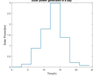
Based on weather forecasting results and solar panel dynamics model, the generated solar power can be estimated. Given a set of parameters of a PV module, such as maximum current and maximum voltage , the power output of a household PV array with 4 parallel strings and 6 series-connected modules per string can be figured out with reference [18], if we assume the PV panel always operates at the maximum power point. Taking the
forecasting results in 3rd July as an example, the daily solar
power curve is estimated as shown in Fig 5. This estimated power curve will be used to evaluate the dynamics and robustness of the energy dispatch scheme in the case study
of this paper.
II. ENERGY BALANCE PROBLEM & PRILIMINARIES
A. Energy balance problem
Considering a standalone microgrid with n-bus system in Fig 1, active power balance excluding transmission loss can be denoted as
∑∈ , − ∑ ∈ , − = 0 (2)
where , are index sets of distributed generators and loads and , and , are distributed power supply and
uncontrollable load demand of the -th and -th units, respectively. Due to the intermittency and uncontrollability of renewable generation and load demand, a proper dispatching strategy is required to share total power mismatch with dispatchable HVAC units , such that
= ∑∈ , − ∑ ∈ , = ∑∈ , (3)
The objective of coordinating multiple HVAC devices is to minimize the power imbalance subjected to power constraints, which is expressed as:
( ) (4a)
. . ∑∈ , = (4b)
, ≤ , ≤ , (4c)
where , and , represent lower and upper power
constraints for the -th HVAC unit, respectively, and is the set of HVAC systems.
B. HVAC model
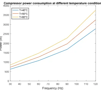
[image:3.595.59.288.221.296.2]A HVAC device is physically composed of a compressor, an evaporator, a condenser, expansion valves, sensors, electrical components and a central controller. With the performance test in [19], [20], Fig 6 demonstrates the relationship between the operating frequency and power consumption when condensation temperature is 40°C, 50°C and 60°C, respectively. As can be seen from the curves, similar trends can be observed under different condensation temperatures, implying that the power consumption is independent with condensation temperature. The relationship between power consumption Figure 3. Identified ES components for all temporal aggregation level.
Figure 4. MAPAx forecasting results
Figure 2. Forecasting results from the multiple linear regression model
Figure 5. A predicted solar power curve in a day
0 5 10 15 20 25
Time(h) 0
0.5 1 1.5 2 2.5
[image:3.595.76.263.435.543.2] [image:3.595.51.285.568.674.2]and compressor frequency can be fitted with a first-order
model as follows:
= , − (5)
where is the frequency of HVAC in bus ; and are a pair of coefficients. By substituting (5) into (3), frequency signals will converge to an optimal value ∗, which is calculated as:
∗= ( − ∑ ) ∑ (6)
The power consumption for each HVAC can be specified as
,∗= ( ∗+ )/ (7)
The above solution can be accomplished by a distributed controller to determine the amount of the power to be assigned to the HVAC devices.
C. Consensus control and graph theory
The communication network among local buses in the microgrid can be assimilated to a multi-agent system. The network is denoted as an undirected graph ( , ℇ), with vertex set = 1, 2, … , and edge set ℇ = ( , )| , ∈
⊆ × . The edge
(
,)
indicates the information exchange between agents and . The neighbour set of the node can be defined as = |(
,)
∈ ℇ . In an undirected graph, the in-degree of a vertex is equal to its out-degree. Mathematically, it can be denoted as == | |, where |
∙
| is the cardinality of a set. The graph iscalled strongly connected if there exists a path between any pair of vertices in the network. The Laplacian matrix =
× is introduced to describe the interaction among
agents based on Vicsek model, which is given as below.
=
, ∈
1 − ∑∈ , =
0, ∉
(8)
It is not difficult to verify that is a positive symmetric matrix and the sum of each column and row is equal to one. Thus, is a doubly stochastic matrix satisfying 1 = 1
and 1 = 1 , where 1 is a column vector with all elements are one.
Suppose ( ) is the state of an agent at time for =
1,2, … , . The consensus problem is to develop a
distributed algorithm, where each agent follows consensus rule and updates its state relying on the information of its neighbours. Eventually all ( ) will converge to a common value about their initial condition. The update rule based on consensus algorithm is written as:
( + 1) = ( ) (9)
As defined above, is associated with a graph. If the undirected graph is strongly connected, then consensus is achievable with the above algorithm, such that
lim
→ ( ) = ∑ (0), as → ∞ for all agents, where
∈ (0,1) is a constant. If = 1/ , it is called average
consensus.
D. MAS-based cooperative control for aggregated
HVACs
In order to address supply-demand imbalance problem, a distributed consensus algorithm is employed to regulate HVAC devices to compensate total power mismatch and to achieve frequency consensus, where an optimal frequency
∗ with power reference
,∗ will be assigned to each
HVAC device.
Define ( ) and ,( ) be compressor frequency and
power consumption for the -th HVAC device at the iteration , respectively. , is the local power mismatch
between the power generation and load demand at bus . is the feedback gain, which dominates the convergence speed. The distributed algorithm in discrete time is described as below:
( + 1) = ∑∈ ( )+ ,( ) (10a)
,( + 1) = ∑∈ , ( ) − ,( + 1) −
,( ) (10b)
,( + 1) = ( ( + 1) + )/ (10c)
The stability of algorithm in eq.(10a) mostly depends on consensus term ∑∈ ( ), which is determined by
communication topology. However, the surplus term
,( ) provides a feedback variable to guarantee the
convergence of the approach. The state feedback gain dominates how fast the state variable , , can converge
to the optimal value ∗, 0, respectively.
The initial condition is given as follow:
(0) = ,(0) −
,(0) ∈ , , ,
,(0) = 0
(11)
Set ,(0) be any value within the power constraints
and total power demand from HVAC is (0) =
∑ ,(0). Eq. (10) can be written as a matrix form:
( + 1) = ( ) + ( ) (12a)
( + 1) = ( ) − ( + 1) − ( ) (12b)
[image:4.595.85.255.90.240.2]( + 1) = ( + 1) + (12c)
where , , are column vectors of , , , , ,
respectively for = 1,2, … , . Define = , =
1/ , = / . Based on the property of
doubly stochastic matrix, we have
1 ( + 1) + ( + 1) = 1 ( ) + ( )
⟹ 1 ( ) + ( ) = ⋯ = 1 (0) + (0)
It indicates that the sum of ( ) + ( ) is a constant for all iteration . Considering the initial condition, we obtain
∑ ,( ) = ∑ ,(0) − ,( ) . If , → 0
when → ∞ for = 1,2, … , , the power mismatch problem can thus be eliminated for each local bus. The eq. (12) can be reformatted as a matrix form
( + 1)
( + 1) = ( )( )
where = ( − ) − (13) Here, the matrix perturbation theory is employed to verify the stability of the presented algorithm under a certain topology. We have the following theorem:
Theorem 1. Suppose a communication network is strongly connected, the average consensus is achievable with distributed algorithm in eq. (10), if the feedback gain is properly small.
In eq. (13), the matrix can be regarded as a deterministic matrix perturbed by a coefficient matrix. The stability proof of Theorem 1 can be referred in [21].
III. SIMULATION RESULTS
This section presents the simulation results to evaluate the feasibility of the proposed algorithm. Then, the solar power forecasting results are integrated into the algorithm to provide a daily energy demand dispatch scheme for the HVAC devices.
As shown in Fig 1, the microgrid is formed by a standard IEEE 5-buses system. Each bus connects a distributed generator, a HVAC unit and uncontrollable load devices. Suppose the microgrid system operates in the standalone mode. The Laplacian matrix can be determined by eq. (8). Table I gives the model coefficients and power constraints of the HVAC devices. The feedback gain matrix is considered as a diagonal matrix to simplify the problem. Suppose that is a constant value and equals to 3.6. Based on eq. (11), initial values are selected as (0) =
[43,56,69,76,116] Hz, (0) = [0, 0, 0, 0,0] kW,
(0) = [1.5, 2.8, 2, 3.5, 3.5] kW, respectively.
A. Case study 1: Feasibility test of the algorithm
In this case, a fixed power mismatch value is given to test the feasibility of the proposed algorithm. Fig 7 shows the update of operating frequency, power consumption, local bus supply-demand power mismatch and total energy
consumption (as demanded to 13.3kW). After 36 iterations, local power mismatch goes to zero, as shown in Fig 7(c), while the power consumed matches the power supplied as shown in Fig 7(d). The operating frequency converges to the optimal value f∗= 72.14 Hz, as indicated in Fig 7(a).
The associated power consumption for each HVAC is
, = 2 kW, , = 3.93 kW, , = 2.135 kW,
, = 3.268 kW and , = 1.96 kW, respectively. It
is worth mentioning that the power of HVAC 1 is saturated after first iteration and those unsaturated HVAC units share more loads to compensate the effect of HVAC 1.
B. Case Study 2: Energy dispatch scheme in a day
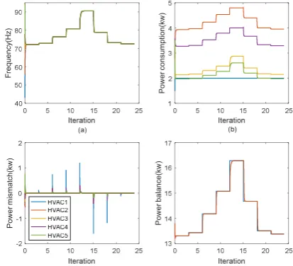
[image:5.595.313.537.199.384.2]This case investigates the performance of the distributed algorithm under time-varying power generation. The simulation results indicate the states of HVAC devices and local bus, based on 24-h solar radiance curve given in Fig 5. Fig 8 (a) and (b) show the dynamics of the operating frequency and power consumption of the HVAC devices in a day. Compared with the Fig 7, the results demonstrate that the proposed distributed algorithm possesses good robustness to overcome the weather uncertainty. The power Figure 7. Simulation results of the consensus algorithm, (a) frequency, (b) HVAC power consumption, (c) estimated power mismatch and (d) power balance
F
requency(H
z)
P
o
w
e
r consum
pti
o
n(kw
)
P
o
w
e
r m
ism
atch(
kw
)
P
o
w
e
r bal
ance(kw
)
TABLEI
PARAMETER SETTING OF THE HVAC UNITS IN MICROGRID SYSTEM
Bus ,(kw) ,(kw) ,( )(kw)
1 17.54 -17.45 2 0.5 1.5
2 14.29 -16 4.8 2 2.8
3 25 -18.75 3.5 0.2 2
4 16.67 -17.67 4 1.6 3.5
[image:5.595.317.524.545.733.2]5 28.57 -15.94 4.5 1 3.5
Fig 8. Simulation results of the consensus algorithm with solar power supply in a day, (a) frequency, (b) HVAC power consumption, (c) estimated power mismatch and (d) power balance
F
requenc
y(
H
z)
Pow
er c
ons
um
pt
ion(k
w
)
P
ow
er
m
ism
at
ch
(k
w
)
Pow
er balanc
e(k
w
mismatch for each local bus converges to zero after each change in the solar power generation, as shown in Fig 8(c). Fig 8(d) shows power consumed exactly matches the power supplied.
IV. CONCLUSIONS
This paper presents an innovative statistical approach in order to forecast a short-term solar radiance curve. Then, an energy dispatch scheme is proposed to dynamically control the power consumption of the HVAC devices to compensate the time-varying effects from the renewable power generation. The case studies have demonstrated the feasibility and robustness of the propose scheme. However, the performance of the forecasting model can be improved by deploying more explanatory variables into the MAPA model, such as dummy variables and lag variables in order to capture data features. Presently, the work focuses on energy balance problem, without consideration of the cooling capacity and comfortable level. An advanced energy dispatch scheme therefore needs to be investigated to achieve these multiple objectives.
ACKNOWLEDGMENT
The authors are grateful to Lancaster Environment Centre for providing solar radiance observation data and Metoffice for providing online weather forecasting data. This work is partly funded by Lancaster University, Centre for Global Eco-Innovation with the partnership of Microgrid Entrust LLP.
REFERENCES
[1] A. Tah and D. Das, “An Enhanced Droop Control Method for Accurate Load Sharing and Voltage Improvement of Isolated and Interconnected DC Microgrids,” IEEE Trans.
Sustain. Energy, vol. 7, no. 3, pp. 1194–1204, 2016.
[2] R. Majumder, A. Ghosh, G. Ledwich, and F. Zare, “Angle droop versus frequency droop in a voltage source converter
based autonomous microgrid,” in 2009 IEEE Power and
Energy Society General Meeting, PES ’09, 2009, pp. 1–8.
[3] S. J. Chiang, C. Y. Yen, and K. T. Chang, “A Multimodule Parallelable Series-Connected,” IEEE Trans. Ind. Electron., vol. 48, no. 3, pp. 506–516, 2001.
[4] J. Miret, M. Castilla, L. GarciadeVicuna, J. Matas, and J. M. uerrero, “A Wireless Controller to Enhance Dynamic Performance of Parallel Inverters in Distributed Generation Systems,” IEEE Trans. Power Electron., vol. 19, no. 5, pp. 1205–1213, 2004.
[5] Y. Han, K. Zhang, H. Li, E. A. A. Coelho, and J. M. Guerrero, “MAS-Based Distributed Coordinated Control and Optimization in Microgrid and Microgrid Clusters: A Comprehensive Overview,” IEEE Trans. Power Electron., vol. 33, no. 8, pp. 6488–6508, 2018.
[6] Y. Han, H. Li, P. Shen, E. A. A. Coelho, and J. M. Guerrero, “Review of Active and Reactive Power Sharing Strategies
in Hierarchical Controlled Microgrids,” IEEE Trans. Power
Electron., vol. 32, no. 3, pp. 2427–2451, 2017.
[7] Y. Xu, W. Zhang, G. Hug, S. Kar, and Z. Li, “Cooperative Control of Distributed Energy Storage Systems in a Microgrid,” IEEE Trans. Smart Grid, vol. 6, no. 1, pp. 238– 248, 2015.
[8] T. Zhao, Z. Zuo, and Z. Ding, “Cooperative control of battery energy storage systems in microgrids,” in
Proceeding of 35th Chinese Control Conference, 2016, pp.
109–120.
[9] T. Morestyn, B. Hredzak, and V. G. Agelidis, “Cooperative Multi-Agent Control of Heterogeneous Storage Devices Distributed in a DC Microgrid,” IEEE Trans. Power Syst., vol. 31, no. 4, pp. 2974–2986, 2016.
[10] V. Trovato, I. M. Sanz, B. Chaudhuri, and G. Strbac, “Advanced Control of Thermostatic Loads for Rapid Frequency Response in Great Britain,” IEEE Trans. Power
Syst., vol. 32, no. 3, pp. 2106–2117, 2017.
[11] J. Hlava and N. Zemtsov, “Aggregated control of electrical heaters for ancillary services provision,” 2015 19th Int. Conf. Syst. Theory, Control Comput. ICSTCC 2015 - Jt.
Conf. SINTES 19, SACCS 15, SIMSIS 19, pp. 508–513,
2015.
[12] S. J. Crocker and J. L. Mathieu, “Adaptive state estimation and control of thermostatic loads for real-time energy
balancing,” in Proceedings of the American Control
Conference, 2016, vol. 2016–July, pp. 3557–3563.
[13] W. Zhang, J. Lian, C. Chang, and K. Kalsi, “Aggregated Modeling and Control of Air Conditioning Loads for Demand Response,” IEEE Trans. Power Syst., vol. 28, no. 4, p. 6415, 2013.
[14] M. Liu and Y. Shi, “Optimal control of aggregated heterogeneous thermostatically controlled loads for regulation services,” in Proceedings of the IEEE Conference
on Decision and Control, 2015, pp. 5871–5876.
[15] J. Ma and X. Ma, “A review of forecasting algorithms and energy management strategies for microgrids,” Syst. Sci.
Control Eng., vol. 6, no. 1, pp. 237–248, 2018.
[16] J. Ma and X. Ma, “State-of-the-art forecasting algorithms for microgrids,” in 23rd IEEE International Conference on
Automation and Computing, 2017, no. September, pp. 7–8.
[17] N. Kourentzes, F. Petropoulos, and J. R. Trapero, “Improving forecasting by estimating time series structural components across multiple frequencies,” Int. J. Forecast., vol. 30, no. 2, pp. 291–302, 2014.
[18] S. Sumathi, L. Ashok Kumar, and P. Surekha, Solar PV and
Wind Energy Conversion Systems. Springer-Verlag, 2015.
[19] Y. C. Park, Y. C. Kim, and M. Min, “Performance analysis on a multi-type inverter air conditioner,” Energy Convers.
Manag., vol. 42, pp. 1607–1621, 2001.
[20] S. Shao, W. Shi, X. Li, and H. Chen, “Performance representation of variable-speed compressor for inverter air conditioners based on experimental data,” Int. J. Refrig., vol. 27, no. 8, pp. 805–815, 2004.