Interpolating Socioeconomic Data for the Analysis of
Deforestation: A Comparison of Methods
Michelle Farfán, Jean François Mas, Laura Osorio
Centro de Investigaciones en Geografía Ambiental, Universidad Nacional Autónoma de México, Morelia, Mexico Email: [email protected]
Received June 8,2012; revised July 8, 2012; accepted August 2, 2012
ABSTRACT
This study compares local-level socioeconomic variables interpolated with three different methods: 1) Thiessen poly-gons, 2) Inverse distance weighting, and 3) Areas of influence based on cost of distance. The main objective was to termine the interpolation technique capable of generating the most efficient variable to explain the distribution of de-forestation through two statistical approaches: generalized linear models and hierarchical partition. The study was con-ducted in two regions of western Mexico: Coyuquilla River watershed, and the Sierra de Manantlan Biosphere Reserve (SMBR). For SMBR it was found that the Thiessen polygons and areas of influence were the techniques that interpo-lated variables with greatest explanatory power for the deforestation process, in Coyuquilla it was inverse distance weighting. These differences are related to the distribution and the spatial correlation of the values of the variables.
Keywords: Interpolation; Socioeconomic Variables; Deforestation;Hierarchical Partition
1. Introduction
Land-use/land-cover changes (LULCC) have become a central question to be addressed in recent years. Vitousek [1] and Agarwal et al. [2] state that the present level of
LULCC constitutes—along with increasing levels of atmospheric carbon dioxide and variations in the global nitrogen cycle—the most evident and perceptible of global changes. Deforestation is known as one of the most important elements of LULCC. According to recent assessments, each year, on average, about 630,000 ha of temperate and tropical forests are cleared, accumulating a total loss of 50% of the original coverage in the last 20 years in Mexico [3]. The Global Forest Resource As-sessment [4] ranks in 4th place the deforestation process in Mexico with an annual loss of 395,000 ha per year from 2000 to 2005. The study of the factors that drive deforestation processes involves not only biophysical but also socioeconomic ones. However, in relation to the second, it is not straightforward to determine which have a greater impact on the processes of change. Some stud-ies consider the demographic aspects as an important cause [5], nevertheless it has also been shown that popu-lation growth is not the main cause of deforestation [6,7]. It is rather a process that depends on a complex combina-tion of socioeconomic and biophysical factors involving the interaction between humans and the environment [8]. In practice, the inclusion of socioeconomic data in de-forestation studies consists in using databases gener-
ated through surveys, which present the data arranged by a specific political-administrative demarcation (state or municipality). Nevertheless, the spatial representation of such units may not reflect their context, as it assumes that they are homogeneous areas to which an average value is assigned. It is therefore advantageous to manage infor-mation by locality, in order to express a greater degree of heterogeneity within each political-administrative de-marcation—from where emerges the challenge of spati-alizing point data by means of some interpolation tech-niques. Geographical information systems (GIS) provide tools to fulfill such task by estimating the values of an environmental variable at unsampled sites using point data from observations within the same region. These methods have been widely used in other environmental matters like soil mapping [9,10] and climatic data [11]. They have also been applied to ecological studies such as the prediction of forest volume [12] and the characteriza-tion of the spatial structure of vegetacharacteriza-tion communities [13].
2. Methods
2.1. Location of Study Areas
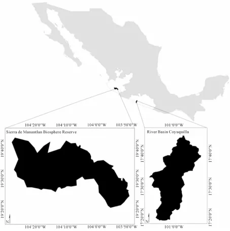
Two study areas were selected: 1) the Sierra de Manant-lan Biosphere Reserve (SMBR) and its area of influence with 4577 km2 in Jalisco; and 2) the Coyuquilla River
watershed, Guerrero, comprising an area of 637 km2 Figure 1).
Figure 1. Location of study areas in Mexico.
2.2. Material
For the SMBR, land-use/land-cover (LULC) data for the year 1970 was obtained from a 1:50,000 scale map pro-duced by the Instituto Nacional de Geografía, Estadística e Informática (INEGI, Mexico’s official mapping agen-cy). This was updated using SPOT images from Decem-ber 2000 and DecemDecem-ber 2004. For the Coyuquilla River watershed, Landsat TM images dated February 1986 and May 2000 were used. In both cases, LULC maps were updated by the visual interdependent interpretation pro-cedure [14,15]. This technique consists first in interpret-ing the image for the first date, and then modifyinterpret-ing it based upon the image for the second date, therefore pro-ducing consistent change data.
The obtained data were used to produce binary maps defining conserved/deforested areas for the aforemen-tioned periods. Random points were then sampled out of each binary map, 40,000 for SMBR and 19,000 for Coyuquilla. Roads maps (scale 1:250,000) and 90-meter resolution digital elevation models (DEM), both from INEGI, were used to generate the friction maps, basic input for the area of influence interpolation technique.
tech-niques were carried out. Statistical analyses were made with R [16].
2.3. Interpolation Techniques
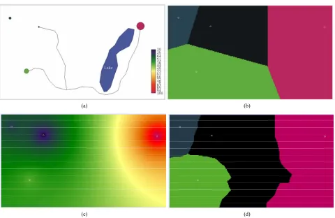
Correlation between the 13 socioeconomic variables from CONAPO (2000) was assessed with the Spearman co- efficient, a non-parametric measure of statistical de- pendence. Variables with a correlation value equal to or greater than 0.7 were discarded. Then, the variables se- lected were spatially interpolated using three methods that are briefly described below. The first method used was Thiessen polygons or Voronoi diagrams. It is based on the Euclidean distance, which divides a region in a way that is totally determined by the configuration of the data points, with one polygon per observation. If the data lie on a regular square grid, then the Thiessen polygons are all equal, but if the data are irregularly spaced, then an irregular lattice of polygons results (see Figure 2(b)).
Each polygon encloses the area closest to the central lo-cation in relation to the distance that keeps with the others to form their boundaries [17]. The entire polygon area receives the value of the attribute of the central point.
The second method is the inverse distance weighting
(IDW), which combines the idea of proximity espoused by the Thiessen polygons with the gradual change of the trend surface. The assumption is that the value of an at-tribute z at some unvisited point is a distance-weighted average of data points occurring within a neighborhood surrounding the unvisited point [18]. Sampled points closer to the unsampled point are more similar to it than those further away in their values [19]. For this study, IDW method was based on 20 and 12 neighboring points for SMBR and Coyuquilla, respectively.
Finally, we generated areas of influence around each locality from Thiessen-like polygons based on friction maps. This is a matrix of cells defining the energy cost for crossing each cell. In this study, the land use map in combination with roads and slope were used as inputs to calculate it. Each area of influence encloses the area closest to the central location in terms of travel time (Figure 2(d)).
2.4. Statistical Comparison of Interpolation Procedure
The performance of each interpolation technique, alone and in combination, was assessed through generalized linear models (GLM), which allow us to develop relationships
(a) (b)
[image:3.595.60.540.386.698.2](c) (d)
Figure 2. Hypothetical interpolation case of four locations. (a) With different attribute values, z, connected by two stretches of road and separated by a lake (barrier) using: Thiessen polygons (b); inverse distance weighted (c) and area of influence (d).
nly the last technique takes into account the road and the lake. O
between the presence/absence of deforestation process and the interpolated variables.
The logistic relation was used since the dependent variable is binary. The statistical support of the GLM is that when the variance is not constant, it is possible to identify the contribution of one or more variables to ex-plain the studied phenomenon. The resulting models were evaluated using the Akaike information criterion (AIC). This criterion incorporates the balance between statistical bias and variance in the factors that are added in the model and provides a comparison directly among themselves [20]. Models were fitted by a step-wise pro-cedure and the relative contribution of each variable was assessed by its significance and the difference of AIC (DAIC) resulting when leaving out the variable from the model.
In addition, hierarchical partitioning (HP) was imple-mented, a protocol in which all possible models in a mul-tiple regression setting are jointly considered to attempt to identify the most likely causal factors. It involves the calculation of the incremental “improvement” (i.e.
in-creased goodness-of-fit) in models by the addition of a given variable U, and these are averaged over all combi-nations in which U occurs to provide a measure of the effects of the independent variables [21]. The independ-ent impact of variable U is estimated by comparing the goodness-of-fit of all possible models involving U. In HP all such comparisons are made and averaged across in-dependent variables and combinations of them in a con-sistent framework. For each independent variable, “ex-planatory” power is segregated into independent effects, I, and effects caused jointly with other variables, J [22,23]. The contribution to the total explained variance of a model of a predictor in conjunction with all others is found by subtracting the total variance explained by a predictor independently. This statistical approach [24] provides a measure of the explanatory power of multiple independent variables because it is not affected by mul-ti-colinearity [25]. MacNally [26] suggests that those
factors identified as influential both in regression models and HP are the causal variables among the ones with predictive power. Finally, the Moran index was calcu-lated to assess the spatial autocorrelation of the variables analyzed.
3. Results
3.1. Selection of the Interpolated Variables
According to the Spearman correlation test, among the 13 socioeconomic variables from CONAPO (2000) only four were found to be not correlated for SMBR and five for Coyuquilla (Table 1).
The selected variables were interpolated through Thi-essen polygons, IDW and areas of influence (Figures 3
and 4), and used in the GLM and HP.
3.2. Comparison of Interpolation Techniques
Table 2 shows the final GLM models for both study
ar-eas with the variables ranked according to the contribu-tion of each variable to the model (DAIC). In general terms, it can be observed that the results of the final GLM model do not produce a consistent way of selecting an interpolation method since it offers a combined selec-tion of mixed techniques. Instead, it was found that, for Coyuquilla as well as SMBR, the variable which exhibits the main contribution was the marginalization index, interpolated with the IDW technique and by Thiessen polygons, respectively.
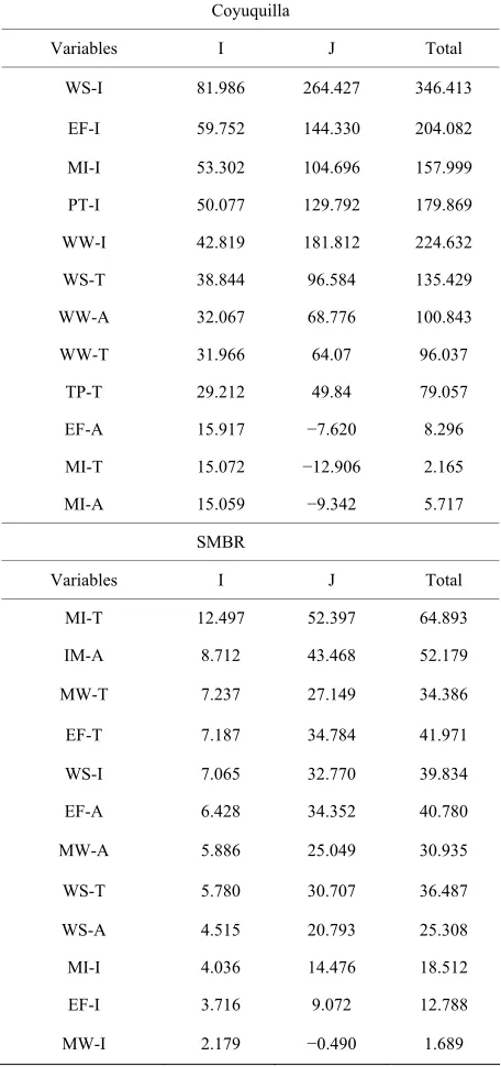
On the other hand the HP results show that for the SMBR the interpolation techniques based on Thiessen polygons and areas of influence are able to spatially ex-press the variables with greater independent explanatory power (I) for the deforestation process (see Table 3).
[image:4.595.60.540.593.731.2]Less important was the IDW technique. It is also possible to observe that the index of marginalization has the highest independent contribution, and in this respect agrees with GLM results. For Coyuquilla, the IDW was
Table 1. Socioeconomic independent variables considered for each study area. The symbol + indicates those variables that were interpolated by 3 methods (Thiessen polygons, IDW and area of influence).
Study area Socioeconomic variables
SMBR Coyuquilla Code
Total population 2000 + TP
% of occupants in houses without sewage or toilet + + WS
% of occupants in homes without running water + WW
% of occupants in houses with earthen floor + + EF
% of employed people with an income up to 2 minimum wages + MW
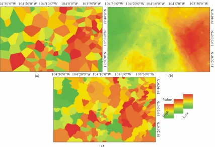
Figure 3. Interpolation of % of employed people with an income up to 2 minimum wages (MW) with, Thiessen polygons (a), IDW (b) and areas of influence (c) for SMBR.
Figure 4. Interpolation of % of occupants in houses with earthen floor (EF) with, Thiessen polygons (a), IDW (b) and areas of nfluence (c) for SMBR.
i
Table 2. GLM final models. Variables which have a higher contribution to the model are expected to exhibit a greater significance (low p-value) and higher value of DAIC. Name codes for variables (see Table 1 for full names) are followed by a letter indicating the interpolation method (I: IDW, T: Thiessen, A: areas of influence).
Coyuquilla SMBR
Variables p-value DAIC Variables p-value DAIC
MI- I 0.000605a 122 MI-T 4.41e−08a 29.3
WS-T 2.0e−16a 34.2 EF-I 0.0000641a 14.9
MI- A 1.79e−08a 22.5 WS-I 0.000247a 13
EF-I 2.0e−16a 16.1 EF-A 0.000549a 11
TP-I 1.38e−16a 15.4 EF-T 0.002065b 8.4
TP-A 0.000492a 13.7 WS-A 0.002466b 8
TP-T 0.344161c 6.5 MW-A 0.005854b 6
EF-T 0.005852b 1.4 MI-I 0.014379c 4.9
WW-I 2.0e−16a 0.3 WS-T 0.033286c 3.5
Significance levels ap < 0.0001, bp < 0.001, cp < 0.01.
the best interpolation technique able to interpolate the socioeconomic variables with more independent contri-bution for explaining the deforestation process. When comparing the results obtained through the HP and GLM approach, it is possible to note that the latter was not able to offer information in terms of selection of one interpo-lation technique and just offered a mix of them.
4. Discussion
The spatial distribution of the values associated with each location can explain why the Thiessen polygons method interpolated “better” the socioeconomic variables for SMBR than the IDW technique used for Coyuquilla.
Figure 5(a) shows how localities with similar values of
marginalization index in the SMBR tend to aggregate in space in a clustered pattern (i.e. with high spatial
auto-correlation, Moran index = 0.65). In contrast, the values of the neighboring localities in the Coyuquilla have con-trasting values without any pattern (low spatial correla-tion, with Moran index = −0.01).
5. Conclusion
[image:6.595.309.537.169.654.2]Socioeconomic local data information is a basic input not only for studies about the drivers of deforestation proc-esses, but also for the purpose of its modeling. None of these studies, however, include as a first step an evalua-tion and selecevalua-tion of the interpolaevalua-tion techniques that are to be used to express the socioeconomic variables. The selection of an appropriate spatial interpolation technique
Table 3. Hierarchical partitioning results with all variables interpolated through the three methods for Coyuquilla and SMBR. Name codes for variables (see Table 1 for full names) are followed by a letter indicating the interpolation method (I: IDW, T: Thiessen, A: areas of influence). The letter I represents the independent contribution, and J is the joint influence in the response variable (deforestation).
Coyuquilla
Variables I J Total
WS-I 81.986 264.427 346.413
EF-I 59.752 144.330 204.082
MI-I 53.302 104.696 157.999
PT-I 50.077 129.792 179.869
WW-I 42.819 181.812 224.632
WS-T 38.844 96.584 135.429
WW-A 32.067 68.776 100.843
WW-T 31.966 64.07 96.037
TP-T 29.212 49.84 79.057
EF-A 15.917 −7.620 8.296
MI-T 15.072 −12.906 2.165
MI-A 15.059 −9.342 5.717
SMBR
Variables I J Total
MI-T 12.497 52.397 64.893
IM-A 8.712 43.468 52.179
MW-T 7.237 27.149 34.386
EF-T 7.187 34.784 41.971
WS-I 7.065 32.770 39.834
EF-A 6.428 34.352 40.780
MW-A 5.886 25.049 30.935
WS-T 5.780 30.707 36.487
WS-A 4.515 20.793 25.308
MI-I 4.036 14.476 18.512
EF-I 3.716 9.072 12.788
MW-I 2.179 −0.490 1.689
(a) (b)
Figure 5. Comparison of marginalization index values in- terpolated with the Thiessen polygons method for the SMBR (a) and Coyuquilla (b).
in the deforestation process by avoiding colinearity pro- blems. This information, combined with spatial autocor-relation analysis based on both feature location and fea-ture value, permits to understand how the data’s spatial distribution is a determining factor in the selection of the interpolator.
6. Acknowledgements
This research was supported by the Consejo Nacional de Ciencia y Tecnología (CONACYT) through grants for the Geography and Biological Sciences graduate pro-grams at UNAM and the project PAPIIT IN113511.
REFERENCES
[1] P. M. Vitousek, “Beyond Global Warming: Ecology and Global Change,” Ecology, Vol. 75, No. 7, 1994, pp. 1861-
1876. doi:10.2307/1941591
[2] C. Agarwal, G. M.Green, J. M. Grove, T. P. Evans and C. M. Schweik, “A Review and Assessment of Land-Use Change Models: Dynamics of Space, Time, and Human Choice,” CIPEC Collaborative Report No.1, Department of Agriculture, Forest Service, Northeastern Research Station, Newton Square, 2002, p. 61.
doi:10.1016/S1364-8152(03)00161-0
[3] J. F. Mas, H. Puig, J. L. Palacio and A. S. Lopez, “Mod- elling Deforestation Using GIS and Artificial Neural Net-works,” Environment Modelling and Software, Vol. 19,
No. 5, 2004, pp. 461-471.
[4] FAO, “Global Forest Resources Assessment 2005: Pro- gress towards Sustainable Forest Management,” FAO Forestry Paper 147, Food and Agriculture Organization of the United Nations, Rome, 2006.
[5] J. C. Allen and D. F. Barnes, “The Causes of Deforesta- tion in Developing Countries,” Annals of the Association of American Geographers, Vol. 75, No. 2, 1985, pp. 163-
184. doi:10.1111/j.1467-8306.1985.tb00079.x
[6] A. Angelsen and D. Kaimowitz, “Rethinking the Causes of Deforestation: Lessons from Economic Models,” World Bank Research Observer, Vol. 14, No. 1, 1999, pp. 73-98.
doi:10.1093/wbro/14.1.73
[7] H. J. Geist and E. F. Lambin, “What Drives Tropical Deforestation? A Meta-Analysis of Proximate and Un- derlying Causes of Deforestation Based on Subnational Scale Case Study Evidence,” LUCC Report Series, No. 4, University of Louvain, Louvainla-Neuve, 2001.
[8] E. F. Lambin, B. L. Turner, J. G. Helmut, et al., “The
Causes of Land-Use and Land-Cover Change: Moving beyond the Myths,” Global Environmental Change, Vol.
11, No. 4, 2001, pp. 261-269. doi:10.1016/S0959-3780(01)00007-3
[9] M. Voltz and R. Webster, “A Comparison of Kriging, Cubic Splines and Classification for Predicting Soil Pro- perties from Sample Information,” Journal of Soil Science,
Vol. 41, No. 3, 1990, pp. 473-490. doi:10.1111/j.1365-2389.1990.tb00080.x
[10] P. I. Booker, “Modeling Spatial Variability Using Soil Profiles in the Riverland of South Australia,” Environ- ment International, Vol. 27, No. 2, 2001, pp. 121-126.
doi:10.1016/S0160-4120(01)00071-X
[11] I. A. Nalder and R. Wein, “Spatial Interpolation of Cli- matic Normals: Test of a New Method in the Canadian Boreal Forest,” Agricultural and Forest Meteorology, Vol. 91, No. 4, 1998, pp. 211-225.
doi:10.1016/S0168-1923(98)00102-6
[12] J. Wallerman, S. Joyce, C. P. Vencatasawmy and H. Ols- son, “Prediction of Forest Steam Volume Using Kriging Adapted to Detect Edges,” Canadian Journal Forest Re- search, Vol. 32, No. 3, 2002, pp. 509-518.
doi:10.1139/x01-214
[13] J. L. Hernandez-Stefanoni and R. Ponce-Hernandez, “Map- ping the Spatial Variability of Plant Diversity in a Tropi- cal Forest: Comparison of Spatial Interpolation Methods,”
Environmental Monitoring and Assessment, Vol. 1, No.
117, 2006, pp. 307-334. doi:10.1007/s10661-006-0885-z
[14] FAO, “Forest Resources Assesment 1990. Survey of Tro- pical Forest Cover and Study of Change Process,” No. 130, Food and Agriculture Organization of the United Nations, Rome, 1996.
[15] F. Achard, H. D. Eva, H. J. Stibin, P. Mayaux, J. Gallego, T. Richards and J. P. Malingreau, “Determination of De- forestation Rates of the World’s Humid Tropical Forests,”
Science, Vol. 297, No. 5583, 2002, pp. 999-1002.
doi:10.1126/science.1070656
[16] R Development Core Team, “R: A Language and Envi- ronment for Statistical Computing. R Foundation for Sta- tistical Computing,” Vienna, 2011.
http://www.R-project.org
[17] P. A. Burrough and R. A. MacDonell, “Principles of Geo- graphical Information Systems (Spatial Information Sys- tems and Geostatistics),” Oxford University Press, Ox-ford, 1998.
[18] J. Li and A. D. Heap, “A Review of Comparative Studies of Spatial Interpolation Methods in Environmental Sci- ences: Performance and Impact Factors,” Ecological In- formatics, Vol. 6, No. 6, 2011, pp. 228-241.
doi:10.1016/j.ecoinf.2010.12.003
and Multimodel Inference,” Springer-Verlag, New York, 2002.
[20] R. Mac Nally, “Regression and Model Building in Con- servation Biology, Biogeography and Ecology: The Dis- tinction between and Reconciliation of ‘Predictive’ and ‘Explanatory’ Models,” Biodiversity and Conservation,
Vol. 9, No. 5, 2000, pp. 655-671. doi:10.1023/A:1008985925162
[21] R. Mac Nally, “Hierarchical Partitioning as an Interpreta-tive Tool in Multivariate Inference,” Australian Journal of Ecology, Vol. 21, No. 2, 1996, pp. 224-228.
doi:10.1111/j.1442-9993.1996.tb00602.x
[22] A. Chevan and M. Sutherland, “Hierarchical Partition-ing,” The American Statistician, Vol. 45, No. 2, 1991, pp.
90-96.
[23] R. Mac Nally and C. J. Walsh, “Hierarchical Partitioning Public-Domain Software,” Biodiversity and Conservation,
Vol. 13, No. 3, 2004, pp. 659-660.
doi:10.1023/B:BIOC.0000009515.11717.0b
[24] R. Mac Nally, “Multiple Regression and Inference in Ecology and Conservation Biology: Further Comments on Identifying Important Predictor Variables,” Biodiver-sity and Conservation, Vol. 11, No. 8, 2002, pp. 1397-
1401. doi:10.1023/A:1016250716679
[25] S. T. Buckland, K. P. Burnham and N. H. Augustin, “Model Selection: An Integral Part of Inference,” Bio- metrics, Vol. 53, No. 2, 2002, pp. 603-618.
doi:10.2307/2533961
[26] M. Baumann, T. Kuemmerle, M. Elbakidze, M. Ozdogan, V. C. Radeloff, N. S. Keuler, A. V. Prishchepov, I. Kruhlov and P. Hostert, “Patterns and Drivers of Post- Socialist Farmland Abandonment in Western Ukraine,”
Land Use Policy, Vol. 28, No. 3, 2011, pp. 552-562.
doi:10.1016/j.landusepol.2010.11.003