On the Estimation of Causality in a Bivariate Dynamic Probit Model on Panel Data with Stata Software: A Technical Review

(1)

ISSN Online: 2162-2086 ISSN Print: 2162-2078

DOI: 10.4236/tel.2018.86083 Apr. 24, 2018 1257 Theoretical Economics Letters

On the Estimation of Causality in a Bivariate

Dynamic Probit Model on Panel Data with

Stata Software: A Technical Review

Richard Moussa

1,2*

, Eric Delattre

1

1_{ThEMA, Université de Cergy-Pontoise,}_{Cergy-Pontoise, France} 2_{ENSEA, Abidjan, Côte D’Ivoire}

Abstract

In order to assess causality between binary economic outcomes, we consider the estimation of a bivariate dynamic probit model on panel data that has the particularity to account the initial conditions of the dynamic process. Due to the intractable form of the likelihood function that is a two dimensions integral, we use an approximation method: The adaptative Gauss-Hermite quadrature method. For the accuracy of the method and to reduce computing time, we derive the gradient of the log-likelihood and the Hessian of the inte-grand. The estimation method has been implemented using the d1 method of Stata software. We made an empirical validation of our estimation method by applying on simulated data set. We also analyze the impact of the number of quadrature points on the estimations and on the estimation process duration. We then conclude that when exceeding 16 quadrature points on our simu-lated data set, the relative differences in the estimated coefficients are around 0.01% but the computing time grows up exponentially.

Keywords

Causality, Bivariate Dynamic Probit, Gauss-Hermite Quadrature, Simulated Likelihood, Gradient, Hessian

1. Introduction

Testing Granger causality has generated a large set of paper in the literature. The larger part of this literature concerns the case where we have continuous dependent variables. For binary outcomes, there is also a way to consider the causality problem. As described by [1] for a vector of dependant variables, the one order Granger causality can be analyse as a probability conditional indepen- How to cite this paper: Moussa, R. and

Delattre, E. (2018) On the Estimation of Causality in a Bivariate Dynamic Probit Model on Panel Data with Stata Software: A Technical Review. Theoretical Economics Letters, 8, 1257-1278.

https://doi.org/10.4236/tel.2018.86083

Received: January 25, 2018 Accepted: April 20, 2018 Published: April 24, 2018 Copyright © 2018 by authors and Scientific Research Publishing Inc. This work is licensed under the Creative Commons Attribution International License (CC BY 4.0).

http://creativecommons.org/licenses/by/4.0/

(2)

DOI: 10.4236/tel.2018.86083 1258 Theoretical Economics Letters

dence given a set of exogenous variables and the first order lagged dependent variables. And for a binary outcome in the dependent vector, one can use a probit probability that implies the use of latent variable.

For panel data case, as the one way fix effects model estimated on a finite sample has necessarily inconsistent estimators [2], the random effect model is used. Due to the fact that we aim to test for one order Granger causality, lagged dependent variables are included as explanatory variables. For the first wave of the panel, we do not have previous values for the dependent variables, and treating them casually or as exogenous leads to inconsistent estimators [2]. So we specify an other equation for initial conditions as described by [3]. The equation is allowed to have different explanatory variables and different idiosyncratic error terms from the dynamic equation.

This specification leads to a likelihood function with an intractable form that is a two dimensions integral with a large set of parameters to be estimated. The estimation of this likelihood function requires the use of numerical approximation of integral function such as maximum simulated likelihood (see [4] for more details) or Gauss-Hermite quadrature (for more details see [5][6][7]).

The main goal of this paper is to propose and to test a method for estimating a two equations system where the explanatory variables are binary in a panel data framework. To the extent of our knowledge, there is no program to do so, especially as we propose the calculation of the Hessian matrix and the gradient vector of our maximisation program.

In this paper, we discuss on the problem of testing Granger causality with a bivariate dynamic probit model taking into account the initial conditions. The organization of this paper is the following one. In Section 2 we explain the causality test method for bivariate probit model with panel data. In Section 3, we describe the estimation method available when the likelihood function has an intractable form (two dimensions integral in our case). Section 4 presents the calculation of the gradient with respect to the model parameters and the calculation of the Hessian matrix with respect to the random effects vector. In Section 5, we present a robustness analysis of our selected estimation method by doing some simulations1_.

2. Testing Causality with a Bivariate Dynamic Probit Model

This section aims to describe causality test method in the case of binary variables. We start by presenting the general approach in time series before introducing panel data case. We end this section by a discussion on the initial conditions problem.

2.1. Testing Causality: General Approach

Causality concept was introduced by [8] as a better predictability of a variable Y

1_{For each section, specifics notations are down at the beginning of the section. Otherwise, in general}

( )x a

(3)

by the use of it lag values, the lag value of an other variable Z and some controls X. In his paper, [8] distinguishes instantaneous causality that means Zt is causing Yt (if Zt is included in the model it improves the predictability of Yt than if not) from lag causality that means lag values of Z improve the predictability of Yt. In this section, we rule out the instantaneous causality and deal with lag causality of one period.

The one period Granger causality can be rephrase in terms of conditional independence. Without lost of generality, we present the univariate case for time series. Let’s Yt and Zt denote some dependent variables and Xt denote a set of controls variables. One period Granger non-causality from Z to Y is the conditional independence of Yt from Zt−1 conditionally to Xt and Yt−1. More

clearly, Granger non-causality from Z to Y is:

(

t| t1, t, t1

)

(

t| t1, t

)

f Y Y₋ X Z₋ = f Y Y₋ X (1) Note that the same kind of relationship can be written for Granger non-causality from Y to Z. As Yt and Zt are binary outcome variables, we can use latent variables ( *

Y and *

Z respectively) and make the assumption that Y and

Z have positive outcomes (equals to 1) if their latent variables are positive. The latent variables are defined as follows:

For the left side of the Equation (1) ( f Y Y

(

t | t−1,X Zt, t−1

)

):

* 1

1 11 1 12 1

t t t t t

Y =X β δ+ Y₋ +δ Z₋ + (2)

* 2

2 21 1 22 1

t t t t t

Z =X β +δ Y₋ +δ Z₋ + (3) For the right side of the Equation (1) ( f Y Y

(

t| t−1,Xt

)

):

* 1

1 11 1

t t t t

Y =Xβ δ+ Y₋ + (4)

* 2

2 21 1

t t t t

Z =X β +δ Z₋ + (5) where

(

)

1

2

1

0, with

1

N ρ

ρ

   

Σ Σ =

   

 



 



 _



To fit the joint distribution of Y and Z conditionally to X (meaning that we estimate a bivariate model), we need to analyze four available situations that are

(

Y= =Z 1

)

,

(

Y = =Z 0

)

,

(

Y=1;Z =0

)

and

(

Y =0;Z =1

)

. For each of these situations, we have:

(

)

(

1 2

)

1 11 1 12 1 2 21 1 22 1

1, 1 |

,

t t t

t t t t t t t t

P Y Z X

P X β δ Y₋ δ Z₋ X β δ Y₋ δ Z₋

= =

=  > − − −  > − − −

(

)

(

1 2

)

1 11 1 12 1 2 21 1 22 1

0, 0 |

,

t t t

t t t t t t t t

P Y Z X

P X β δ Y₋ δ Z₋ Xβ δ Y₋ δ Z₋

= =

=  < − − −  < − − −

(

)

(

1 2

)

1 11 1 12 1 2 21 1 22 1

1, 0 |

,

t t t

t t t t t t t t

P Y Z X

= =

=  > − − −  < − − −

(

)

(

1 2

)

1 11 1 12 1 2 21 1 22 1

0, 1 |

,

t t t

t t t t t t t t

P Y Z X

= =

(4)

As we can see, by assuming 1

2 1

t t

q = Y − and q_t2=2Z_t−1, we can rewrite the probabilities above as:

(

)

(

) (

)

(

1 2 1 2

)

2 1 11 1 12 1 2 21 1 22 1

, |

, ,

t t t

t t t t t t t t t t

P Y Z X

q X β δ Y₋ δ Z₋ q X β δ Y₋ δ Z₋ q q ρ

= Φ + + + + _ (6)

where Φ2

( )

stands for the bivariate normal c.d.f.

Then testing Granger non-causality in this specification is testing

12

0 : 0

H δ = for Z is not causing Y and testing H0 :δ =21 0 for Y is not causing

Z.

2.2. Testing Causality: Panel Data Case

For panel data case, two major approaches can be used. The first one is to consider that causal effect is not the same for all individuals in the panel ([9]). This approach is useful when individuals are heterogeneous or when the causal effect is not homogeneous. The specification for latent variables are:

* 1 1 1

1 11, , 1 12, , 1

it t i i t i i t i it

Y =X β δ+ Y ₋ +δ Z ₋ +η ζ+ (7)

* 2 2 2

2 21, , 1 22, , 1

it t i i t i i t i it

Z =X β +δ Y ₋ +δ Z ₋ +η +ζ (8) where

(

1 2

)

, i i

η η ′_{denotes the individual random effects which are zero mean and}

covariance matrix Ση and

(

ζ ζ ′it1, it2

)

denote the idiosyncratic shocks which are zero mean and covariance matrix Σζ with

2

1 1 2

2

1 2 2

1 and

1 ζ η

η ζ

ζ η

ρ

σ

σ σ ρ

ρ

σ σ ρ

σ

   

Σ =_ _ Σ = 

 

In this approach, testing Granger non-causality is equivalent to test 12,i 0,i 1, ,N

δ = = _ _for_Z_{is not causing}_Y_{and to test}δ_21,_i =0,i=1,,N for Y is not causing Z.

The second approach (that is used in this paper) is to assume the causal effects, if they exist, are the same for all individuals in the panel. With the same notation that the previous case, the latent variables are:

* 1 1 1

1 11 , 1 12 , 1

it t i t i t i it

Y =X β δ+ Y ₋ +δ Z ₋ +η ζ+ (9)

* 2 2 2

2 21 , 1 22 , 1

it t i t i t i it

Z =X β +δ Y ₋ +δ Z ₋ +η +ζ (10) Then testing Granger non-causality is equivalent to test H0 :δ =12 0 for Z is

not causing Y and to test H0 :δ =21 0 for Y is not causing Z.

Finally, Equations (9) and (10) are the core of our problem. Since Y and Z are binary panel outcomes and each equation includes lag dependent variables, estimating jointly these two equations can be viewed as the estimation of a bivariate dynamic probit model.

2.3. Dealing with Initial Conditions

For the first wave of the panel (initial conditions), due to the fact that we do not have data for the previous state on Y and Z (no values for Yi,0 and Zi,0) we are

(5)

of the panel. This means that they assume the data generating process of the first wave of the panel to be exogenous or to be in equilibrium. These assumptions hold only if the individual random effects are degenerated. If this assumption is not fulfilled, the initial conditions (the first wave of the panel) are explained by the individual random effects and ignoring them leads to inconsistent parameter estimates [2].

The solution proposed by [2] for the univariate case and generalized by [3] is to estimate a static equation for the first wave of the panel (meaning that we do not introduce lagged dependent variables). In this static equation, the random effects are a linear combination of the random effects in the next wave of the panel and idiosyncratic error terms may have different structure from the idiosyncratic error terms in the dynamic equation. Formally, the latent variables for the first wave of the panel are defined as follows:

* 1 1 2 1

,1 1 11 12

i i i i i

Y =X γ +λ η +λ η + (11)

* 2 1 2 2

,1 2 21 22

i i i i i

Z =X γ +λ η +λ η + (12) where

( )

1 2

, i i

′

  denotes the vector of idiosyncratic shocks which are zero mean and covariance matrix Σ__with 1

1 ρ ρ

 

Σ =  

 

 



.

As η1 and η2 are individual random effects respectively on Y and Z,

12

λ

and

λ

21 can be interpreted as the influence of the Y random individual effects (respectively Z random individual effects) on Z (respectively on Y) at the first wave of the panel.

3. Estimation Methods

Due to the fact that the likelihood function has an intractable form (an integral function), it is impossible to estimate this likelihood by usual methods. We then deal with numerical integration methods that are numerical approximation method for an integral. In this section we describe two major methods and argue for one of them to estimate our likelihood function.

3.1. Gauss-Hermite Quadrature Method

The Gauss-Hermite quadrature is a numerical approximation method use to close the value of an integral function. The default approach is related to an univariate integral of the form:

( )

_exp

( )

2 _d

f x −x x

∫

(13) where _exp

( )

₋_x2 _{denotes the Gaussian factor}2_{. Then the integral above can be} approximated using:

( )

2

( )

1

exp d

Q

q q

q

f x x x w f x

=

− =

∑

∗

∫

 (14)

2_{Notice that even without this factor, one can use the Gauss-Hermite quadrature by using a}

straightforward transformation that is to multiply and divide the integrand f x( ) by a Gaussian factor

( )

2

(6)

where x q_q, =1,,Q are nodes from the Hermite polynomial and

, 1, ,

q

w q=  Q are corresponding weights.

This approximation supposes that the integrand can be well approximated by an 2Q+1 order polynomial and that the integrand is sampled on a symmetric

range centered on zero. So, for suitable results, these two assumptions must be taken into account.

We first assume that finding the optimal number of quadrature points can be achieved numerically. For the accuracy of the approximation, it is required to choose the optimal number of quadrature points. To do this, one can start with a number q of quadrature points and increase it to assess if it significantly

changes the result, and repeat this process until convergence in terms of overall likelihood value variation and estimated coefficients variation. But, it is also important to take into account the fact that increasing number of quadrature points also increases the computing time. An example of the impact of number of quadrature points on estimated results is given in Section 5.

For the problem of suitable sampling range, the solution of using the adaptative Gauss-Hermite quadrature was proposed by [5] and [6]. In this approach, instead of using

( )

2

exp −x as a Gaussian factor, they use a Gaussian density

(

2

)

,

φ µ σ _{of mean}_μ_{and variance}_σ2_{. That means (see}_[5]_):

( )

*

1

d Q

q q

q

f x x w f x∗

=

∑

∫

 (15)

Then the sampling range is transformed and the new nodes are *

2

q q

x = +µ σx and weights are w_q* = 2σw_qexp

( )

x2_q . For [5], one can choose the normal density with posterior mean and variance equal respectively to μ and σ2_{. For the implementation, we can start with}_{µ =}₀_and _σ ₌₁_{and at each} iteration of the likelihood maximization process, calculate the posterior weighted mean and variance of the quadrature points and use them to calculate the nodes and weights for the next iteration. For [6], one can choose μ to be the mode of the integrand f x

( )

and σ to be the square of the Hessian of the log of

integrand taken in the mode.

( )

(

)

1 2

2

ˆ

log

x x

f x x

σ

−

=

 _∂ 

= −_ _

∂

  (16) For the multivariate integral case, the same approach is used. Without lost of generality, we discuss the bivariate case that can be apply to others multivariate cases. The function to approximate is written as follows:

(

)

2f x y, d dx y

∫

 (17)

With the assumption of independence between x and y (that can be overcome by using a Cholesky decomposition x′ =x and y′=ρx′+y, see [5] or [7] for

more precision on these Cholesky transformation or other transformations that can lead to similar results) the integral above can be approximated by:

( )

(

)

2 1 2 1 1

1 2

* * * *

1, 1

, d d ,

Q

q q q q

q q

f x y x y w w f x y

= =

=

∑

(7)

And in this case, the nodes and weights are derived as follows:

( )

(

)

1

1 1

1 2

* ₂

2 *

ˆ ,

ˆ 2 log , q

q

q x y x

x x

x f x y

y x

y

−

=

 

  _∂  

 

  = + ∗ − ∗_ _

   ∂  _ _

    (19)

and

( )

(

)

( )

1 1

1

2 ₂ ₂

1 2 ₂

* ₂

2

* ₂

ˆ ,

exp

2 log ,

exp

q q

q

q x y x q q

w x

w

f x y x

w w x

−

=

 

  _∂ _ _

  = ∗ − ∗

  ∂  

  _ _ (20)

where A denotes the determinant of matrix A, and xˆ denotes the mode of

the integrand f x y

(

,

)

.

Jackel (2005) also suggests that for the nodes with low weights (when contributions to the integral value are not significant) we can prune the range from those nodes in order to save calculation time. That means to set a scalar

( )

1 Q1 2 w w

Q

τ +

= _{and drop all nodes with weights lower than this scalar.}

3.2. Maximum Simulated Likelihood Method

Maximum Simulated Likelihood method was introduced by [4] as a solution to maximization problems that have an integral as objective function. In this approach, the likelihood function is supposed to be defined as:

( )

2

(

) (

)

*

1 2 1 2 1 2

, , , , , d d

f x y =

∫

f x y u u g u u u u

 (21)

where g u u

(

1, 2

)

is a probability distribution function,

(

)

*

1 2

, , ,

f x y u u is called simulator and denotes the function from which the mean value at some draws u1 and u2 gives an approximation of the overall likelihood. Without lost of generality, we only define the two dimensions case that can be generalized to fewer or larger dimensions integral. For this kind of likelihood function, [4] proposed as simulator the function *

(

)

1 2

, , ,

f x y u u with u1 and u2 drawn from the same probability distribution function g (the probability distribution function of the individual random effects). Then the overall likelihood function can be approximated by (u1d denotes the dth_{draw from}_u_{1; the same definition} holds for u2d):

( )

*

(

)

1 2

1

, , , ,

D

d d

d

f x y f x y u u

D =

=

∑

₍₂₂₎

where D denotes the number of draws.

To implement this method, we start by simulating a bivariate normal draw

(

0, 2

)

(8)

The simulated likelihood estimator is consistent and asymptotically equivalent to the likelihood estimator ([4]) if the number of draws tend to infinity faster than N .

3.3. GHQ or MSL: What Method to Choose?

As described above, they are two main methods to estimate our likelihood function. To choose which method to implement, we deal with the accuracy and the computing time requirement.

For our estimations, we choose the adaptative Gauss-Hermite quadrature proposed by [7] for three main reasons.

 _{Our dataset is an unbalanced panel data with 10,569 individuals observed in} mean over 26 years, that leads 255,206 observations. Due to the fact that the simulated likelihood method requires that the number of draw D be larger than the square of the number of observations, we do not use it to avoid waste of time in computing process.

 The Gauss-Hermite quadrature requires that we find the best number of quadrature Q that is the one for whom the integrand can be well approximated by an 2Q+1 order polynomial. If Q is small, that reduces

computing time. Our estimations are achieved in general for Q between 8 and 14. It means that at each iteration, for the likelihood value calculation, we do a weighted sum of between 2

8 =64 and 142=196 terms.

 _{Using the Gauss-Hermite quadrature method reduces computing time but} this computing time remains very long if the integrand is not sampled at the suitable range (meaning that the adaptative method has not been used). And in this case, the maximization process spends between two and three weeks before achieving convergence on an Intel Core i7 computer at 3.4 GHz with 8 GB of RAM memory. By applying the adaptative Gauss-Hermite quadrature, the computing time is significantly reduced and then, we spend between two and three days for achieving convergence on the same computer.

(9)

4. Chosen Method Requirements

In this section we describe some requirements of the selected method that is the adaptative Gauss-Hermite Quadrature. The first one is the fact that the adaptative Gauss-Hermite quadrature requires to derive the Hessian of the log of the integrand ([6]). The second one is that we derive the gradient of the overall likelihood function in order to use Stata’s d1 method (see [10]) for more accuracy and more speed in the calculations.

4.1. Gradient Vector Calculation

The gradient of the overall log-likelihood function has been calculated to speed up the maximization process. This will allow us to use the Stata’s d1 method that requires the implementation of the gradient vector in addition to the log-likelihood. The likelihood function for an individual i is:

(

)

(

)

(

)

2

1 0 2 0 1 2 1 2 1 2 1 2

2 0 0 0 0 2

2

, , , , , d d

i

T

i i i i i i i it it it it it it i i i

t

L q h q w q q ρ q h q w q q ρ φ η_ζ _η η η

=

_∫

Φ

∏

Φ Σ

  (23)

where

1 1

2 1 ,

it it

q = y − ∀i t

2 ₂ 2 ₁ _,

it it

q = y − ∀i t

0 1 1 2

1 11 12

i i i i

h =Zγ +λ η +λ η

0 2 1 2

2 21 22

i i i i

w =Z γ +λ η +λ η

1 1

1 11 , 1 12 , 1

it it i t i t i

h =X β δ+ h ₋ +δ w ₋ +η

2 2

2 21 , 1 22 , 1

it it i t i t i

w =X β +δ h ₋ +δ w ₋ +η

Using the adaptative Gauss-Hermite quadrature method by [6], the overall likelihood function is given by (we use the same notation that those used in Section 3):

(

)

(

)

(

)

1 * 2 *

* * 1 0 2 0 1 2

2 0 0 0 0

1, 1

1 2 1 2

2

, 2

, ,

, , ,

i

i k i j

Q

i k j i i i i i i

k j

T

it it it it it it i

x x

t

L w w q h q w q q

q h q w q q _ζ _{η η}

η ρ

ρ φ η

= =

=

= Φ

× Φ Σ

∑

∏



(24)

To get the gradient vector, the log-likelihood above must be derived with respect to 13 parameters that are: β1=

(

β δ δ1, 11, 12

)

′, β2=

(

β δ δ2, 21, 22

)

′, γ1, γ2,

11

λ , λ12, λ21, λ22, σ1, σ2, ρη, ρζ , and ρ.

Let’s lkj denotes:

(

)

(

)

(

)

1 * 2 *

1 0 2 0 1 2 1 2 1 2

2 0 0 0 0 2

, 2

, , , , ,

i

i k i j

T

kj i i i i i i it it it it it it i

x x

t

l q h q w q q ρ q h q w q q ρ φ ηζ _{η η}₌ _η ₌

=

= Φ _

∏

Φ Σ

Then, the first order derivatives with respect to each α of the 13 parameters is given by:

( )

1, 1

log Q

kj i

k j i

l L

L α

α = =

∂ ∂

∂

=

(10)

With respect to β1 the first order derivative is:

( )

(

)

2 2

1 1

1 ₂

1 2 1 2

2

1 2

1

, ,

i

it it it it

it it it T

kj kj

t _{it it} _it _it _it _it

q w q h

q q h l

l

q h q w q q ζ ζ ζ ρ φ ρ

β = ρ

 ₋    Φ  ₋  ∂ _ _ =

∂

∑

Φ

With respect to β2 the first order derivative is:

(

)

(

)

1 1

2 2

1 ₂

1 2 1 2

2

2 2

1

, ,

i

it it it it

it it it

T kj

kj

t _{it it} _it _it _it _it

q h q w

q q w

l l

q h q w q q ζ ζ ζ ρ φ ρ

β = ρ

 ₋    Φ  ₋  ∂ _ _ =

∂

∑

Φ

With respect to γ1 the first order derivative is:

(

)

(

)

2 0 2 0

1 1 0 0 0

0 0 1 ₂

1 0 2 0 1 2

1 2 0 0 0 0

1

, ,

i i i i

i i i

kj kj

i i i i i i

q w q h

q q h

l l

q h q w q q

ρ φ ρ γ ρ  ₋    Φ  ₋  ∂ _ _ = ∂ Φ   

With respect to γ2 the first order derivative is:

(

)

(

)

1 0 1 0

2 2 0 0 0

0 0 1

2

1 0 2 0 1 2

2 2 0 0 0 0

1

, ,

i i i i

i i i

kj kj

i i i i i i

q h q w

q q w

l l

q h q w q q

ρ φ ρ γ ρ  ₋    Φ  ₋  ∂ _ _ = ∂ Φ   

With respect to λ11 the first order derivative is:

(

)

(

)

2 0 2 0

1 * 1 0 0 0

0 0 1 ₂

1 0 2 0 1 2

11 2 0 0 0 0

1

, ,

i i i i

i k i i kj

kj

i i i i i i

q w q h

q x q h

l l

q h q w q q

ρ φ ρ λ ρ  ₋    Φ  ₋  ∂ _ _ = ∂ Φ   

(

)

(

)

2 0 2 0

1 * 1 0 0 0

0 0 1 ₂

1 0 2 0 1 2

12 2 0 0 0 0

1

, ,

i i i i

i j i i kj

kj

i i i i i i

q w q h

q x q h

l l

q h q w q q

ρ φ ρ λ ρ  ₋    Φ  ₋  ∂ _ _ = ∂ Φ   

(

)

(

)

1 0 1 0

2 * 2 0 0 0

0 0 1

2

1 0 2 0 1 2

21 2 0 0 0 0

1

, ,

i i i i

i k i i

kj kj

i i i i i i

q h q w

q x q w

l l

q h q w q q

ρ φ ρ λ ρ  ₋    Φ  ₋  ∂ _ _ = ∂ Φ   

(

)

(

)

1 0 1 0

2 * 2 0 0 0

0 0 1

2

1 0 2 0 1 2

22 2 0 0 0 0

1

, ,

i i i i

i j i i

kj kj

i i i i i i

q h q w

q x q w

l l

q h q w q q

(11)

With respect to σ1 the first order derivative is:

( )

(

)

(

)

2

* * *

1 1 2

2 1

1

log 1

k k j

kj kj

x x x

l

l η

η

σ ρ σ σ

σ ρ  ₋  ∂ _ _ = ∗ − +_ _ ∂ _ − _  

With respect to σ2 the first order derivative is:

( )

(

)

(

)

2

* * *

2 1 2

2 2

1

log 1

j k j

kj kj

x x x

l

l η

η

σ ρ σ σ

σ ρ  ₋  ∂ _ _ = ∗ − +_ _ ∂ _ − _  

With respect to ρη the first order derivative is:

(

) (

)

(

_* 2 _* 2

)

(

₂

)

_* _*

(

)

1 2 1 2

1 2 2

1

1 1

log 1

k j k j

kj

x x x x

l l η η η η η η

ρ σ σ ρ σ σ

ρ ρ ρ ρ  ₊ _{− +}  ∂   = ∗_ − _ −  +    ∂ _ _   −  

With respect to ρζ the first order derivative is:

(

)

(

)

1 2 1 2 1 2

2 ₂ , , , , 1 log 1 i T

it it it it it it it it kj

kj

t _{it it} _it _it _it _it

q q q h q w q q

l

q h q w q q

ζ ζ ζ ζ φ ρ ρ ρ ρ = ∂ = Φ  +  ∂ _ _ −  

∑

With respect to ρ__{the first order derivative is:}

(

)

(

)

1 2 1 0 2 0 1 2

0 0 0 0 0 0

1 2 1 0 2 0 1 2

2 0 0 0 0

, ,

1 log

1

i i i i i i i i

kj

i i i i i i

q q q h q w q q l

l

q h q w q q

φ ρ ρ ρ ρ ∂ = Φ  +  ∂ _ _ −       Remarks:

• For σ1, σ2, ρη , ρζ , and ρ, we used some transformations on

parameters to insure that in the maximization process, each σ remains positive and each ρ remains between −1 and 1 at all iteration. For σ we use exponential transformation then in the derivation, we derive with respect to

( )

log σ . For ρ we use arc-tangency transformation (i.e.

( )

exp 2 1

ρ ρ

−

+ ) then in the derivation, we derive with respect to

1 2 1 log 1 ρ ρ  +   ₋    .

• To easily derive a bivariate normal probability with zero mean, variance one and correlation ρ, we can transform it into an integral where the integrand is a product of an univariate normal density and an univariate normal probability as follows:

(

)

( )

2 , , ₂ d ₂ d .

1 1

y x v x y u

x y ρ φ v ρ v φ u ρ u

ρ ρ

−∞ −∞

 ₋   ₋ 

   

Φ = Φ = Φ

 ₋   ₋ 

   

∫

(12)

(

)

_{( )}

2

, ,

1

x y y x

x x

ρ _φ ρ

ρ

 

∂Φ _ − _

= Φ

 

∂ _ ₋ _

(

)

_{( )}

2

, ,

1

x y x y

y y

ρ _φ ρ

ρ

 

∂Φ _ − _

= Φ_ _

∂ _ ₋ _

4.2. Hessian Matrix Calculation

For the requirement of the adaptative Gauss-Hermite quadrature method, we need to derive the Hessian matrix of the log of the integrand function with respect to the random effects vector3_{. From the individual likelihood function} defined in Equation 23, the log of the integrand is:

(

)

(

)

(

)

(

)

(

)

1 2

1 0 2 0 1 2 1 2 1 2

2 0 0 0 0 2

2

log ,

log , , , , ,

i

i i

T

i i i i i i it it it it it it i

t

g

q h q w q q q h q w q q _ζ _η

η η

ρ ρ φ η

=

 

= _Φ Φ Σ _

 

∏



(25)

We derive from the log of the integrand in Equation (25) the Hessian matrix by calculating:

( )

(

)

2

1 2

2

1 log i, i

i

g η η

η ∂ −

∂

( )

(

)

2

1 2

2

2 log i, i

i

g η η

η ∂ −

∂

(

)

(

)

2

1 2

1 1log i, i

i i

g η η

η η ∂ −

∂ ∂

The first order derivatives are given by:

( )

(

)

(

)

(

)

(

)

1 2 1 2

1 0 2 0 1 2

2

2 0 0 0 0

1 0 2 0 1 2 1 2 1 2

2

2 0 0 0 0 2

1 2 2

1 1 2

2

, ,

log

, , , ,

1

i

T

it it it it it it

i i i i i i

t

i i i i i i i it it it it it it

i i

q h q w q q q h q w q q

g

ζ

η

ρ ρ

η ρ ρ

η σ ρη σ σ

ρ

=

′

′ Φ

Φ ∂

− = − −

∂ Φ Φ

− +

−

∑

 

With respect to 1

i

η we have:

(

)

(

)

(

)

1

2 0 2 0

1 0 2 0 1 2 1 1 0 0 0

0 0 0 0 0 11 0 1

2 2

1 0 1 0

2 2 0 0 0

0 21 0 1 ₂

, ,

1

i

i i i i

i i i i i i i i i

i i i i

i i i

q w q h

q h q w q q q q h

q h q w

q q w

η

ρ

ρ λ φ

ρ

ρ λ φ

ρ

 ₋ 

 

′

Φ = Φ

 ₋ 

 

 ₋ 

 

+ Φ

 ₋ 

 

 

  

3_{In this section,}_φ( )_x _{denotes the univariate normal density function,}_φ(_{x y}_{, ,}_ρ)_{denote the}

(13)

(

)

( )

1

2 2

1 2 1 2 1 1

1

2 , , 2

1

i

it it it it it it it it it it it it it

q w q h

q h q w q q ζ q q h ζ

η ζ ρ ρ φ ρ  ₋    ′

Φ = Φ

 ₋ 

 

And with respect to 2

i

η we have:

(

)

(

)

(

)

2

2 0 2 0

1 0 2 0 1 2 1 1 0 0 0

0 0 0 0 0 12 0 1

2 2

1 0 1 0

2 2 0 0 0

0 22 0 1 ₂

, ,

1

i

i i i i

i i i i i i i i i

i i i i

i i i

q w q h

q h q w q q q q h

q h q w

q q w

η

ρ

ρ λ φ

ρ ρ λ φ ρ  ₋    ′

Φ = Φ

 ₋     ₋    + Φ  ₋        

(

) (

)

2 1 1

1 2 1 2 2

1

2 , , 2

1

i

it it it it it it it it it it it it

q h q w

q h q w q q ζ q w ζ

η ζ ρ ρ φ ρ  ₋    ′

Φ = Φ

 ₋ 

 

The second order derivatives are given by:

( )

(

) (

)

(

)

(

)

(

)

1 1 1

1 0 2 0 1 2 1 0 2 0 1 2 2

0 0 0 0 2 0 0 0 0

2

2 2 1 0 2 0 1 2

1

2 0 0 0 0

2 1 0 2 0 1 2

0 0 0 0

2

2 1 0 2 0 1 2

2 0 0 0 0

1 2 2 2 , , , , log , , , , , , , , i i i i

i i i i i i i i i i i i

i i i i i i

i

i i i i i i

T

it it it it it

t

g

q h q w q q

q h q w q η η η ρ ρ ρ η ρ ρ = ′′ Φ Φ ∂ − = − Φ ∂ ′ Φ + Φ ′′ Φ −

∑

    

(

) (

)

(

)

(

)

(

)

(

)

1

1 2 1 2 1 2

2

2 1 2 1 2

2

2 1 2 1 2

2

2 2

2 1 2 1 2

1 2

, ,

, , ₁

1

, ,

i

it it it it it it it

it it it it it it

q q h q w q q

q h q w q q

ζ ζ ζ ζ η η ζ ρ ρ ρ ρ σ ρ ρ  _Φ   _Φ   ′ Φ  − +  ₋ Φ _ (26)

( )

(

) (

)

(

)

(

)

(

)

1 2 2 2

1 0 2 0 1 2 1 0 2 0 1 2 2

0 0 0 0 2 0 0 0 0

2

2 2 1 0 2 0 1 2

2

2 0 0 0 0

2 1 0 2 0 1 2

0 0 0 0

2

2 1 0 2 0 1 2

2 0 0 0 0

1 2 2 2 , , , , log , , , , , , , , i i i

i i i i i i

i

i i i i i i

T

it it it it it

t

g

q h q w q q

q h q w q η η η ρ ρ ρ η ρ ρ = ′′ Φ Φ ∂ − = − Φ ∂ ′ Φ + Φ ′′ Φ −

∑

    

(

) (

)

(

)

(

)

(

)

(

)

2

1 2 1 2 1 2

2

2 1 2 1 2

2

2 1 2 1 2

2

2 1 2 1 2 2 2

2 1

, ,

, , ₁

, , 1

i

it it it it it it it

it it it it it it

q q h q w q q

q h q w q q

ζ ζ ζ ζ η ζ η ρ ρ ρ ρ

ρ σ ρ

 Φ   _Φ   ′ Φ  − + 

Φ _ −

(27)

( )

(

) (

)

(

)

(

)

(

)

1 2 1 2

1 0 2 0 1 2 1 0 2 0 1 2 2

0 0 0 0 2 0 0 0 0

2

1 2 2 1 0 2 0 1 2

2 0 0 0 0

1 0 2 0 1 2 1 0 2 0 1 2

0 0 0 0 0 0 0 0

2 2

2 1 0 2 0 1 2

2 0 0 0 0

, , , ,

log

, ,

, , , ,

, ,

i i i i i i i i i i i i i i

i i i i i i i i

i i i i i i

g

q h q w q q

q h q w q q ε η η

η η

ρ ρ

η δη ρ

ρ ρ ′′ Φ Φ ∂ − = − ∂ Φ ′ ′ Φ Φ + Φ    

(

)

(

) (

)

(

)

1 2

1 2 1 2 1 2 1 2

2 2

2 1 2 1 2

2 ₂ , , , , , , i i i T

it it it it it it it it it it it it

t _it _it _it _it _it _it

q h q w q q

ζ ζ η η ζ ρ ρ ρ ρ =

 ′′Φ Φ

(14)

(

)

(

)

(

)

(

)

1 2

1 2 1 2 1 2 1 2

2 2

2 1 2 1 2

2 2 1 2 , , , , , , 1

it it it it it it it it it it it it

it it it it it it

q h q w q q

ζ ζ η η ζ η η ρ ρ ρ ρ

σ σ ρ

 ′ ′ Φ Φ  −  Φ _ − − (28) where

(

)

(

)

(

)

1 1 1

1 2 1 2

2

1 2 1 2 1 2 1 2

2

, ,

, , , ,

i

i i

it it it it it it

it it it it it it it it it it it it it

q h q w q q

h q h q w q q q h q w q q

ζ η

ζ ζ ζ

η η

ρ

ρ ρ φ ρ

′′ Φ

′

= − Φ −

(

)

(

)

(

)

2

2 1

1 2 1 2

2

1 2 1 2 1 2 1 2

2

, ,

, , , ,

i

i i

it it it it it it

it it it it it it it it it it it it it

q h q w q q

w q h q w q q q h q w q q

ζ η

ζ ζ ζ

η η

ρ

ρ ρ φ ρ

′′ Φ

′

= − Φ −

(

)

(

)

1 2 1

1 2 1 2 1 2 1 2 1 2

2i i it it, it it, it it it it i it it, it it, it it

q h q w q q _ζ q q q h q w q q _ζ

η η ρ ρζφη ρ

′′ Φ =

(

)

(

)

(

)

(

)

(

)

(

)

1

1 0 2 0 1 2

0 0 0 0

2

2 2 1 0 2 0 1 2

11 21 11 21 0 0 0 0

2 0 2 0

2 0 1 0 0 0

11 0 1 ₂

1 0 1 0

2 0 2 0 0 0

21 0 1

2

, ,

2 , ,

1

i i i i i i i

i i i i i i

i i i i

i i i

i i i i

i i i

q h q w q q

q w q h

h q h

q h q w

w q w

η

ε

ε ρ

λ λ ρ λ λ φ ρ

ρ λ φ ρ ρ λ φ ρ ′′ Φ = − +  ₋    − Φ  ₋     ₋    − Φ  ₋        

(

)

(

)

(

)

(

)

(

)

(

)

2

1 0 2 0 1 2

0 0 0 0

2

2 2 1 0 2 0 1 2

12 22 12 22 0 0 0 0

2 0 2 0

2 0 1 0 0 0

12 0 1

2

1 0 1 0

2 0 2 0 0 0

22 0 1 ₂

, ,

2 , ,

1

i i i i i i i

i i i i i i

i i i i

i i i

i i i i

i i i

q h q w q q

q w q h

h q h

q h q w

w q w

η

ε ρ

λ λ ρ λ λ φ ρ

ρ λ φ ρ ρ λ φ ρ ′′ Φ = − +  ₋    − Φ  ₋     ₋    − Φ  ₋         

(

)

(

)

(

)

(

)

(

)

(

)

1 1

1 0 2 0 1 2

0 0 0 0

2

1 2 1 0 2 0 1 2

0 0 11 22 12 21 11 12 21 22 2 0 0 0 0

2 0 2 0

0 1 0 0 0

11 12 0 1 ₂

1 0 1 0

0 2 0 0 0

21 22 0 1

2

, ,

1

i i i i i i i i

i i i i i i i i

i i i i

i i i

i i i i

i i i

q h q w q q

q q q h q w q q

q w q h

h q h

q h q w

w q w

η η ρ

λ λ λ λ ρ λ λ λ λ φ ρ

ρ

λ λ φ

ρ

λ λ φ

ρ ′′ Φ = + − +  ₋    − Φ  ₋     ₋   − Φ  ₋           

Then, the Hessian matrix is given by:

( )

2 2

2 1 2

1

2 2

1 2 ₂ 2

log log

i i i

i i _i

g g

H

g g

η η η

η δη _η

(15)

As described in Section 3.1, after having derived this Hessian matrix, we calculate its value at the mode of the integrand and use it to re-sample the integrand.

5. Robustness Analysis Based on Simulations

This section aims to insure that the implemented method gives suitable results. We consider that the implemented method give us suitable results if for a given relationship between variables, by applying the estimation method on these variables we find approximatively the same coefficients. To reach this goal, we perform a robustness analysis on the estimation method. This robustness analysis is an empirical one based on simulations. We use two different approaches for that.

The first approach is to simulate bivariate binary variables by specifying a relationship between some explanatory variables (it means that we set coefficients of explanatory variables) and estimate this relationship with the implemented method in order to compare the results with the relationship specified before. In the second approach, we introduce new variables (that were not used in the data generating process) when estimating the relationship with the implemented method and compare the new results with the first ones. The implemented method is robust when it is able to correctly estimate the relationship specified even if we introduce other variables and also to estimate non significant coefficients to those other variables. Finally, the method we make use of to check for the robustness is the same that in [11].

As the estimation method implemented is a numerical approximation method, the results will depend on the selected number of quadrature points. We deal with the incidence of number of quadrature points on results in the last part of this section. For a better analysis of the results we also add the standard errors of each estimated coefficients.

5.1. Simulated Relationship between Real Variables

In this section, we use variables from the French SIP (Santé et Itinéraire Professionnel) survey data set and we simulate error terms and a relationship between some selected variables. The subset of the database use for this section is an unbalanced panel of 1202 individuals with total waves per individual between 5 and 10 waves.

We set the error terms parameters as σ =1 2.1, σ =2 3.1, ρη =0.7 ,

0.5 ζ

ρ = _and ρ =_ 0.4.

We simulate idiosyncratic errors vectors ζ =

(

ζ ζ1, 2

)

′ and =

(

 1, 2

)

′ as bivariate normal variables with zero mean, variance equal to 1 and covariances respectively equal to ρζ and ρ. We also simulate individual random effects

as bivariate normal variables with zero mean, covariance equals to ρη and variance equals to 2

1

σ for the first component of the random effects vector and equals to 2

2

(16)

( )

1=rnormal 0,1



( )

2

2=rnormal 0,1 ∗ 1−

ρ

 +

ρ

1

 

( )

1 rnormal 0,1

ζ =

( )

2

2 rnormal 0,1 1 ζ ζ 1

ζ = ∗ −ρ +ρ ζ

where rnormal

(

µ σ,

)

denote the random normal density with mean μ and standard deviation σ. As individuals effects are time invariant, we simulate η as follows:

(

)

1 rnormal 0, 1 ift 1

η = σ =

(

)

2 2

2 2 1

1

0, 1 if 1

rnormal _η _ησ t

η σ ρ ρ η

σ

= ∗ − + =

[

]

1 1 t 1 if t 1

η η= = ≠

[

]

2 2 t 1 if t 1

η =η = ≠

For the initial conditions (t=1), the simulated relationship is the following:

*

1 0.2 0.3 0.2 0.4 1 0.5 2 1 y = − + ill− unemp+ η − η +

*

2 2 0.2 0.08 0.3 1 0.5 2 2 y = − ill− age+ η + η +

(

*

)

1 1 0

y = y >

(

*

)

2 2 0

y = y >

For t>1, we specify the following relationship:

*

1t 1.9 0.3 1, 1t 0.1 2, 1t 0.05 t 0.2 t 1 1t

y = + y ₋ + y ₋ − Male − unemp + +η ζ

*

2t 0.4 0.11, 1t 0.4 2, 1t 0.05 t 0.5 t 2 2t

y = − − y ₋ + y ₋ + Male − dens +η +ζ

(

*

)

1t 1t 0

y = y >

(

*

)

2t 2t 0

y = y >

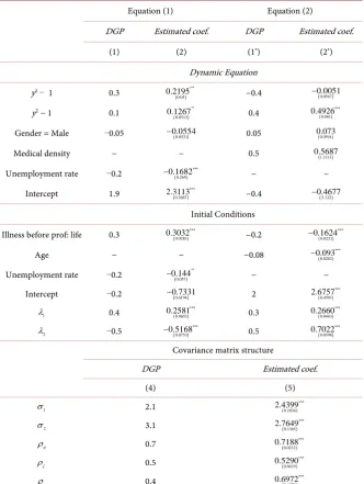
The variable ill denotes having an illness episode in the year, unemp denotes being out of labour marking during the year, age denotes the age of individual, and Male is 1 if individual is male and 0 otherwise. Estimation results for 16 quadrature points are displayed in Table 1. For all equations, we give the coefficients that are used in the DGP and those that are estimated by our program. As we can see, all the coefficients from the DGP are very closed from the estimates ones.

5.2. Simulated Relationship with Additional Variables

(17)

[image:17.595.207.540.89.531.2]

Table 1. Simulated data set estimation’s results.

Equation (1) Equation (2)

DGP Estimated coef. DGP Estimated coef.

(1) (2) (1’) (2’)

Dynamic Equation

y1₋ ₁ _0.3

(0.05)

0.2195∗∗∗ _−0.4 ₍ ₎

0.0567 0.0051 −

y2_{− 1} _0.1

(0.0513)

0.1267∗∗ _0.4 ₍ ₎***

0.061 0.4926

Gender = Male −_0.05 −0.0554₍_0.0521₎ _0.05 ₍ ₎ 0.0594 0.073

Medical density − − 0.5 0.5687(1.1111)

Unemployment rate −_0.2 ₍ ₎ *** 0.269 0.1682

− ₋ ₋

Intercept 1.9 ( )

*** 0.2667

2.3113 _−0.4 ₍ ₎

2.122 0.4677 −

Initial Conditions Illness before prof: life 0.3 ( )

*** 0.0283

0.3032 _−0.2 ₍ ₎***

0.0221 0.1624 −

Age − − −0.08 ( )

*** 0.0202 0.093 −

Unemployment rate −_0.2 ₍ ₎

0.057 0.144∗∗

− ₋ ₋

Intercept −_0.2 −0.7331₍_0.6194₎ ₂ ₍ ₎***

0.4591 2.6757

1

λ 0.4 ( )

*** 0.0651

0.2581 _0.3 ₍ ₎***

0.0463 0.2660

2

λ −_0.5 ₍ ₎***

0.0753 0.5168

− _0.5

( )

*** 0.0598 0.7022

Covariance matrix structure

DGP Estimated coef.

(4) (5)

1

σ 2.1 ( )

*** 0.1034 2.4399

2

σ 3.1 ( )

*** 0.1365 2.7649

η

ρ 0.7 ( )

*** 0.0212 0.7188

ζ

ρ _0.5 ₍ ₎***

0.0419 0.5290

ε

ρ 0.4 ( )

*** 0.1378 0.6972

Estimated standard deviations for estimated coefficients are given within parenthesis. ***: significant at the 1% level, **: significant at the 5% level.

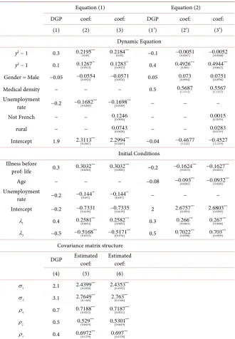
significant. We introduce two variables rural and nationality (notFrench) in the dynamic equations of the regression.

Results are in Table 2. Columns 1 and 2 in Table 2 are the same than corresponding columns in Table 1. We provide in Table 2, column 3, the new results with the additional variables in order to compare with previous estimates4_. As we can see in the Table 2, the coefficients estimated (using again 16 quadrature points) for those variables are not significant and all initial coefficients in the model remain approximately the same.

4_{We do the same with columns 1’, 2’ of}_{Table 1}_and_{Table 2}_{(new results are in column 3’) and with}

(18)

[image:18.595.208.539.87.564.2]

Table 2. Simulated data set with added variables estimation’s results.

Equation (1) Equation (2)

DGP coef: coef: DGP coef: coef:

(1) (2) (3) (1’) (2’) (3’)

Dynamic Equation y1_{− 1} _0.3

( )

*** 0.05

0.2195 ₍ ₎*** 0.05

0.2184 _−0.1 ₍ ₎

0.0567 0.0051

− ₍ ₎

0.0568 0.0052 −

y2_{− 1} _0.1

( )

** 0.0513

0.1267 ₍ ₎** 0.0513

0.1283 _0.4 ₍ ₎*** 0.061

0.4926 ₍ ₎*** 0.0612 0.4944

Gender = Male −0.05 −0.0554(0.0521) −0.0571(0.0521) 0.05 0.073(0.0594) 0.0751(0.0596) Medical density − − − 0.5 0.5687(1.1111) 0.5567(1.1112) Unemployment

rate −0.2 ( )

*** 0.0269 0.1682

− ₍ ₎***

0.0269 0.1698

− ₋ ₋ ₋

Not French − − 0.1246(0.0956) − − 0.0015(0.1076)

rural − − 0.0743(0.0628) − − 0.0283(0.0719)

Intercept 1.9 ( )

*** 0.2667

2.3113 ₍ ₎*** 0.2667

2.2994 _−0.04 ₍ ₎

2.122 0.4677

− ₍ ₎

2.1215 0.4527 −

Initial Conditions Illness before

prof: life 0.3 ( )

*** 0.0283

0.3032 ₍ ₎*** 0.0283

0.3032 _−0.2 ₍ ₎*** 0.0221 0.1624 −

( )

*** 0.0221 0.1627 −

Age − − − −0.08 ( )

*** 0.0202 0.093

− ₍ ₎***

0.0202 0.0932 −

Unemployment

rate −0.2 ( )

** 0.057 0.144

− ₍ ₎**

0.057 0.144

− ₋ ₋ ₋

Intercept −0.2 −0.7331(0.6194) −0.7335(0.6195) 2 ( ) *** 0.4591

2.6757 ₍ ₎*** 0.4595 2.6803

1

λ 0.4 ( )

*** 0.0651

0.2581 ₍ ₎*** 0.0653

0.2582 _0.3 ₍ ₎*** 0.0463

0.266 ₍ ₎*** 0.0464 0.267

2

λ _−0.5 ₍ ₎***

0.0753 0.5168 −

( )

*** 0.0754 0.5171

− _0.5

( )

*** 0.0598

0.7022 ₍ ₎*** 0.0599 0.703

Covariance matrix structure DGP Estimated _coef: Estimated _coef:

(4) (5) (6)

1

σ 2.1 ( )

*** 0.1034

2.4399 ₍ ₎*** 0.1032 2.4353

2

σ 3.1 ( )

*** 0.1365

2.7649 ₍ ₎*** 0.1366 2.763

η

ρ _0.7 ₍ ₎***

0.0212

0.7188 ₍ ₎*** 0.0212 0.7187

ζ

ρ 0.5 ( )

*** 0.0419

0.529 ₍ ₎*** 0.0419 0.5301

ε

ρ _0.4 ₍ ₎***

0.1379

0.6972 ₍ ₎*** 0.1378 0.697

Estimated standard deviations for estimated coefficients are given within parenthesis. ***: significant at the 1% level. **: significant at the 5% level.

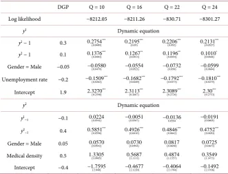
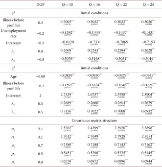
5.3. Impact of Number of Quadrature Points on Estimated Results

As the accuracy of the method depends on the number of quadrature points used for the likelihood calculation, we propose an assessment of how it affects the results when this number increases. For doing so, we fit the same model with different numbers of quadrature points and we calculate the relative difference in log-likelihood and in estimated parameters.