Star formation histories of z~1 galaxies in LEGA C

STAR FORMATION HISTORIES OFZ ∼1 GALAXIES IN LEGA-C

Priscilla Chauke,1 Arjen van der Wel,2, 1 Camilla Pacifici,3 Rachel Bezanson,4 Po-Feng Wu,1 Anna Gallazzi,5

Kai Noeske,6 Caroline Straatman,2 Juan-Carlos Mu˜nos-Mateos,7 Marijn Franx,8 Ivana Bariˇsi´c,9

Eric F. Bell,10 Gabriel B. Brammer,3 Joao Calhau,11 Josha van Houdt,9Ivo Labb´e,8 Michael V. Maseda,8

Adam Muzzin,12Hans-Walter Rix,9and David Sobral8, 11

1_{Max-Planck-Institut f¨ur Astronomie, K¨onigstuhl 17, D-69117 Heidelberg, Germany} 2_{Sterrenkundig Observatorium, Universiteit Gent, Krijgslaan 281 S9, B-9000 Gent, Belgium}

3_{Space Telescope Science Institute, 3700 San Martin Drive, Baltimore, MD 21218, USA}

4_{University of Pittsburgh, Department of Physics and Astronomy, 100 Allen Hall, 3941 O’Hara St, Pittsburgh PA 15260, USA} 5_{INAF-Osservatorio Astrofisico di Arcetri, Largo Enrico, Fermi 5, I-50125 Firenze, Italy}

6_{Experimenta Heilbronn, Kranenstraße 14, 74072, Heilbronn, Germany}

7_{European Southern Observatory, Alonso de Cordova 3107, Casilla 19001, Vitacura, Santiago, Chile} 8_{Leiden Observatory, Leiden University, PO Box 9513, 2300 RA Leiden, The Netherlands}

9_{Max-Planck Institut f¨ur Astronomie, K¨onigstuhl 17, D-69117, Heidelberg, Germany}

10_{Department of Astronomy, University of Michigan, 1085 S. University Ave., Ann Arbor, MI 48109, USA} 11_{Physics Department, Lancaster University, Lancaster LA1 4YB, UK}

12_{Department of Physics and Astronomy, York University, 4700 Keele St., Toronto, Ontario, MJ3 1P3, Canada}

Submitted to ApJ

ABSTRACT

Using high resolution spectra from the VLT LEGA-C program, we reconstruct the star formation histories (SFHs) of 607 galaxies at redshiftsz= 0.6−1.0 and stellar masses_&1010M using a custom

full spectrum fitting algorithm that incorporates the emcee and FSPS packages. We show that the mass-weighted age of a galaxy correlates strongly with stellar velocity dispersion (σ∗) and ongoing

star-formation (SF) activity, with the stellar content in higher-σ∗ galaxies having formed earlier and

faster. The SFHs of quiescent galaxies are generally consistent with passive evolution since their main SF epoch, but a minority show clear evidence of a rejuvenation event in their recent past. The mean age of stars in galaxies that are star-forming is generally significantly younger, with SF peaking after z <1.5 for almost all star-forming galaxies in the sample: many of these still have either constant or rising SFRs on timescales > 100 Myrs. This indicates thatz > 2 progenitors of z ∼ 1 star-forming galaxies are generally far less massive. Finally, despite considerable variance in the individual SFHs, we show that the current SF activity of massive galaxies (>L∗) atz∼1 correlates with SF levels at least

3 Gyrs prior: SFHs retain ‘memory’ on a large fraction of the Hubble time. Our results illustrate a novel approach to resolve the formation phase of galaxies, and in identifying their individual evolutionary paths, connects progenitors and descendants across cosmic time. This is uniquely enabled by the high-quality continuum spectroscopy provided by the LEGA-C survey.

Keywords: galaxies: star formation histories — galaxies: high-redshift — galaxies: evolution

1. INTRODUCTION

The ability to reconstruct the star-formation histories of galaxies, by characterising their stellar populations, allows one to trace their individual evolution through

chauke@mpia-hd.mpg.de

star-formation histories (SFHs) and how these are related to global galaxy properties. To constrain galaxy forma-tion theories more directly, ‘archaeological’ reconstruc-tion can be used to trace the evolureconstruc-tion of individual galaxies over time, and then the dependance of individ-ual SFHs on stellar mass, stellar velocity dispersion and star-formation (SF) activity can be explored.

Reconstructing SFHs requires high resolution spectra of galaxies. Ideally, individual stars would be resolved, as they are for local dwarf galaxies (e.g., Weisz et al. 2011). However, in most cases we have to rely on in-tegrated stellar light, though if a galaxy’s main star formation (SF) epoch lies at z > 1, we cannot tem-porally resolve its stellar age distribution, even with the highest-quality spectra. While there is a plethora of high resolution spectra of galaxies in the local uni-verse, most of these galaxies are too old (>5 Gyrs, Gal-lazzi et al. 2005) to resolve their star-formation histories (SFHs) due to the similarity of stellar spectra in the age range>5 Gyrs. The general insight gained from the ‘ar-chaeological’ studies of these galaxies is that low-mass galaxies have more extended SFHs that peak at later cosmic times compared to high-mass galaxies (‘downsiz-ing’, e.g.,Gallazzi et al. 2005;Thomas et al. 2005,2010). Many of these studies involved the use of fossil record methods on SDSS (Sloan Digital Sky Survey,York et al. 2000) spectra of local galaxies (e.g. Juneau et al. 2005;

Thomas et al. 2005; Cid Fernandes et al. 2007; Tojeiro et al. 2009; McDermid et al. 2015; Ibarra-Medel et al. 2016). However, downsizing has also been seen in other studies, such as studies by Cimatti et al. (2006), who corrected luminosity function data of early-type galax-ies by adopting the empirical luminosity dimming rate derived from the evolution of the Fundamental Plane of field and cluster massive early-type galaxies, as well as Leitner (2012), who derived the average growth of stellar mass in local star-forming galaxies using a Main Sequence Integration approach.

One approach to probe the high-redshift regime, is to obtain an integrated view of galaxy evolution. Thus far, this has been the focus of spectroscopic observations of distant galaxies: the evolution of the star-formation rate density (SFRD) in the universe has been exten-sively studied (e.g.,Karim et al. 2011;Madau & Dickin-son 2014;Khostovan et al. 2015;Abramson et al. 2016). The majority of these studies indicate that the SFRD increased from high redshift to z ∼ 2, and has since been decreasing steeply. Coupled with this, are num-ber density evolution studies which show an increasingly dominant population of quiescent galaxies (e.g.,Pozzetti et al. 2010;Brammer et al. 2011;Moustakas et al. 2013;

Muzzin et al. 2013a).

Another approach is to use photometric measurements to trace SFHs, however, individual galaxy evolution is not easily traced with this method due to high uncer-tainties. In this case, one can investigate average SFHs of galaxies asPacifici et al.(2016) have done by apply-ing spectral energy distribution models to compute the median SFHs of 845 quiescent galaxies at 0.2< z <2.1. They found that galaxy stellar mass is a driving factor in determining how evolved galaxies are, with high mass galaxies being the most evolved at any time. The limi-tation with these approaches is that we cannot connect progenitors to descendants: studies from mass-matched samples have resulted in multiple solutions (e.g.,Torrey et al. 2017). To understand the mechanics of how galax-ies evolve, it is crucial to expand our view from focusing on the population of galaxies as a whole, to investigating how the star-formation rate (SFR) of individual galaxies varies with time.

Probing the SFHs of individual galaxies, however, still requires high-resolution, high-quality stellar continuum spectra, which are expensive to obtain. Consequently, high-redshift samples are small and often selected with criteria to optimize data quality and sample size rather than represent the full galaxy population. Jørgensen & Chiboucas (2013) obtained spectra for ∼80 cluster galaxies atz= 0.5−0.9 and found ages of 3−6 Gyrs, consistent with passive evolution between z ∼ 2 and the present. Stellar population measurements of ∼ 70 z∼0.7 galaxies with stellar masses>1010Mwere

popu-lation, which is arguably justified for very massive galax-ies at late cosmic epochs, but not in general.

The LEGA-C (Large Early Galaxy Astrophysics Cen-sus, van der Wel et al. 2016) survey is collecting high S/N spectra of ∼ 3000 galaxies in the redshift range 0.6 <z<1, selected only by theirK-band magnitude (a proxy for stellar mass). The data, which are compa-rable in quality to those obtained in the nearby universe, probe the internal kinematics of stars and gas, and the ages and metallicities of stellar populations. This en-ables us, for the first time, to reconstruct the SFHs of individual galaxies at large look-back time that are representative of the population. These reconstructed SFHs can provide a direct connection between progeni-tors and descendants, and allow us to constrain when, and how quickly, galaxies formed their stars.

Over the past decade, there have been several al-gorithms developed to recover SFHs, viz. MOPED,

STARLIGHT,STECMAP,VESPA,ULYSS and

FIRE-FLY (Heavens et al. 2000; Cid Fernandes et al. 2005;

Ocvirk et al. 2006;Tojeiro et al. 2007;Koleva et al. 2009;

Wilkinson et al. 2015). We develop our own approach in this study to tailor the problem for galaxies atz∼1. The main differences between our algorithm and some of those listed above are the use of composite stellar populations (a group of stars which range in age within a given interval) instead of simple stellar populations (stars born from a single burst in star formation); using a defined set of template spectra which allow for di-rect comparisons of the SFHs; as well as the assumption of constant star formation within a given time interval. The galaxy spectra are also not continuum-normalised in the fitting process, but photometry is used to cali-brate the fluxes.

The goal of this paper is to reconstruct the SFHs of galaxies in the LEGA-C sample and investigate the de-pendance of individual SFHs on stellar mass, stellar ve-locity dispersion and star-formation (SF) activity. The paper is outlined as follows. In Section 2 we give a brief overview of the LEGA-C dataset. In Section 3we introduce the model for reconstructing the SFHs of the galaxies as well as tests of the model. In Section4 we present a sample of the resultant fits and general trends of measured parameters. In Section 5 we investigate the SFH as a function of stellar velocity dispersion and stellar mass. We demonstrate that we can verify the re-lation between the evolution of SFHs and mass, and we investigate the variation in the reconstructed SFHs, at fixed stellar velocity dispersion. Finally, in Section5we summarise the results. A ΛCDM model is assumed withH0= 67.7 km s−1Mpc−1, Ωm= 0.3 and ΩΛ= 0.7.

2. DATA

LEGA-C (van der Wel et al. 2016) is an ongoing ESO Public Spectroscopic survey with VLT/VIMOS of ∼3000 galaxies in the COSMOS field (R.A.= 10h₀₀m_;

Dec. = +2◦120). The galaxies were selected from the Ultra-VISTA catalog (Muzzin et al. 2013b), with red-shifts in the range 0.6 < z < 1.0. The galaxies were K-band selected with a magnitude limit ranging from K(AB) = 21.08 at z = 0.6 to K(AB) = 20.7 at z = 0.8 to K(AB) = 20.36 at z = 1.0 (stellar masses M∗ > 1010M). These criteria were chosen to

re-duce the dependence on variations in age, SF activ-ity and extinction, as well as ensure that the targets were bright enough in the observed wavelength range (0.6µm−0.9µm) to obtain high quality, high resolution spectra (R∼3000). Each galaxy is observed for∼20 h, which results in spectra withS/N∼20 ˚A−1_.

The analyses in this work are based on the first-year data release1, which contains spectra of 892 galaxies, 678 of which are in the primary sample and have a S/N > 5 ˚A−1 _{between rest-frame wavelengths 4000 ˚A}

and 4300 ˚A (typically, S/N ∼ 20 ˚A−1). Emission line subtracted spectra are used in the fitting algorithm; therefore, the emission line spectrum of each galaxy, computed using the Penalized Pixel-Fitting method (pPXF, Cappellari & Emsellem 2004), is subtracted from the observed spectrum. For details of the emission line fitting procedure, see Bezanson et al. (2018, sub-mitted to ApJ). As part of the analysis of the model, we use the following measured quantities: stellar ve-locity dispersions (σ∗), 4000 ˚A break (Dn4000) and Hδ

equivalent width indices [EW(Hδ)], U-V colours, stellar masses (M∗,F AST), UV+IR SFRs, and UV+IR specific

SFRs (sSFRU V+IR). Stellar masses are determined

using FAST (Kriek et al. 2009) based on photometric measurements, Bruzual & Charlot(2003) stellar popu-lation libraries, adopting aChabrier(2003) Initial Mass Function (IMF), Calzetti et al. (2000) dust extinction, and exponentially declining SFRs. The UV+IR SFRs are estimated from the UV and IR luminosities, fol-lowing Whitaker et al. (2012). For details of the data reduction procedure, seevan der Wel et al.(2016).

3. SPECTRAL FITTING TECHNIQUE

3.1. Stellar Population Model

To reconstruct the SFHs of galaxies, one needs to gauge the various ages of stellar populations within these galaxies. This is done using stellar population spectra generated with the Python implementation of the

Table 1. Properties of theFSPStemplate spectra.

Age Bina SFRb M∗c Lbold

log(yr) M/yr M log(L)

0.000−8.000 1.000×10−8 0.837 1.964 8.000−8.300 1.005×10−8 _{0.711 0.885}

8.300−8.475 1.010×10−8 0.748 0.650 8.475−8.650 6.750×10−9 _{0.731 0.497}

8.650−8.750 8.646×10−9 0.718 0.382 8.750−8.875 5.332×10−9 _{0.707 0.285}

8.875−9.000 3.998×10−9 0.695 0.187 9.000−9.075 5.305×10−9 0.685 0.127 9.075−9.225 2.040×10−9 _{0.671 0.099}

9.225−9.375 1.444×10−9 0.652 −0.043 9.375−9.525 1.022×10−9 _{0.639 −0.161}

9.525−9.845 2.681×10−10 0.618 −0.347

a_{Age interval of CSP templates.}

b_{SFR s.t. 1 M}

of stars formed within the interval.

c_{Stellar mass (including stellar remnants) with}

mass loss accounted for.

d_{Bolometric luminosity.}

3000 3500 4000 4500 5000

Wavelength [ ]

0 1 2 3 4 5 6 7

Flux

Age in log(yr)

age: 0.0 - 8.0 age: 8.0 - 8.3 age: 8.3 - 8.5 age: 8.5 - 8.7

age: 8.7 - 8.8 age: 8.8 - 8.9

age: 8.9 - 9.0

age: 9.0 - 9.1 age: 9.1 - 9.2 age: 9.2 - 9.4 age: 9.4 - 9.5

age: 9.5 - 9.8

Figure 1.Template CSP spectra used to fit LEGA-C galax-ies. They were generated fromFSPS, using the time intervals listed in Table1, with solar metallicity and arbitrary velocity dispersion; and they have been normalised and shifted here for comparison purposes.

ible Stellar Population Synthesis package (FSPS v3.0;

Conroy & Gunn 2010; Conroy et al. 2009; Foreman-Mackey et al. 2014), using the MILES spectral library (S´anchez-Bl´azquez et al. 2006), Padova isochrones ( Gi-rardi et al. 2000; Marigo & Girardi 2007; Marigo et al. 2008) and a Kroupa initial mass function (Kroupa et al. 2001).

A galaxy spectrum is approximated to be a linear com-bination of template spectra at varying ages, attenuated by dust:

fλ= n

X

i=1

miTλ,i10−0.4kλE(B−V)i, (1)

kλ= 2.659

−2.156 + 1.509

λ −

0.198 λ2 +

0.011 λ3

+ 4.05

wherenis the number of stellar population spectra to fit to the galaxy,Tλ,i are the template spectra,mi are the

weights that scale the templates to match the spectra of the galaxy,kλ is the reddening curve (Calzetti et al.

2000), andE(B−V)i are the dust reddening values.

We generate 12 composite stellar population spectra (CSPs), with solar metallicity (see Section3.3), covering ages from 0 to about 7 Gyrs, the age of the Universe in LEGA-C’s redshift range. To determine the intervals of the 12 age bins of the CSPs, simple stellar population spectra (SSPs) were generated and the cumulative abso-lute difference from one spectrum to another was calcu-lated as the age was increased; which was then divided into 12 percentiles with equal width (see Table 1 and Figure1for the properties of the CSPs in each age bin). This method of determining the time intervals generates template spectra that optimise the temporal sampling of an evolving stellar population. In practice, the age bins are∼0.15 dex wide over the age range 0−7 Gyrs.

The template spectra are generated with a constant SFR and are normalised such that 1 M of stars are

8.0

8.5

9.0

9.5

log(Age[yr])

0

20

40

60

80

100

120

SF

R

[M

/yr

]

S/N = 10

Galaxy SFH

Reconstructed SFH

8.0

8.5

9.0

9.5

log(Age[yr])

0

20

40

60

80

SF

R

[M

/yr

]

S/N = 30

Galaxy SFH

Reconstructed SFH

Figure 2. Reconstructed SFH (black) of a synthetic galaxy (green) with S/N = 10 ˚A−1 (left) and S/N = 30 ˚A−1 (right). The converged walkers are shown in grey and the upper and lower uncertainties are based on the 16th and 84th percentiles, respectively, as explained in Section 3.2. By S/N = 30 ˚A−1_{, the recovered SFHs predict the stellar mass, age and luminosity}

with precision≤0.1 dex.

clouds (Charlot & Fall 2000). Therefore, two dust red-dening values are fit for: E(B−V)1, for the age range

0−100 Myrs, and E(B−V)2, for the rest of the age

ranges.

3.2. Fitting Algorithm

To find the optimal values for the 14 parameters, viz. the 12 weight factors (mi) for the 12 CSP templates and

2 dust reddening values (E(B−V)i), we usedemcee, a

Python implementation of an affine invariant ensemble sampler for MCMC (Foreman-Mackey et al. 2013) which was proposed by Goodman & Weare (2010). It uses MCMC ‘walkers’ which randomly explore the parame-ter space, where each proposed step for a given walker depends on the positions of all the other walkers in the ensemble, with the aim of converging to the most likely parameter values.

The priors for the 14 parameters were set such that all parameter values were always greater or equal to 0, and the upper limit forE(B−V)iwas set to 3. The

pa-rameter value for the youngest bin was initially set to be equal to the measured SFR from UV+IR measurements, but it was allowed to vary between 1/3 and 3 times that value during the fitting process, allowing for measure-ment errors. For the other bins, the best fitting sin-gle template, computed using least-squares fitting, was assigned all the stellar mass, with all other parameter values set to 10−6. Starting with equal SFRs in all bins also recovers the SFHs, however, the algorithm may take longer to converge to the optimal values.

For each galaxy, 100 MCMC walkers were used, initi-ated in a small region around the starting values men-tioned above. A total of 20000 samples were taken and 1000 steps were kept after burn-in. The mean accep-tance fraction was_&0.2 and the typical autocorrelation time was ∼ 95 iterations. The optimal values for the parameters are taken as the 50th _{percentile of the list}

of samples of the converged walkers, and the lower and upper uncertainties are the 16th and 84th percentiles, respectively. The fitting algorithm resulted in 607 good fits based on their normalised χ2 _{values (<5, from}

vi-sual inspection of the fits), and these were used in the analyses. The spectra that were not well-fit were mainly due to low S/N and AGN.

3.3. Robustness of Fitting Results

To assess the robustness of the model, we performed the following tests: generate and fit synthetic spectra; compare model stellar mass measurements of the LEGA-C population with those obtained from broad-band pho-tometry (see Section2); fit a sample of SDSS spectra and compare model stellar masses with literature measure-ments; and test the assumption of solar metallicity.

Synthetic galaxy spectra were generated with varying SFHs using the CSPs in Section 3.1, including simu-lated noise that mimics LEGA-C variance spectra, to compare how well the algorithm recovered the SFHs. 20 SFHs were generated for each S/N (5, 10, 20, 30, 40, 50 and 60 ˚A−1), and the average deviations of the true a<M W >, stellar mass and luminosity from the

the model sufficiently recovered the SFHs, however, we note that the quality of the results depends on the noise introduced into a spectrum (see Figure2 for two exam-ples). Stellar mass and luminosity are recovered with precision≤0.1 dex for S/N≥20, while a<M W > only

re-quires S/N≥10 to reach the same level of precision. We note that these tests only constrain the purely random uncertainties due to the noise in the spectra while they do not include systematic errors in the data (e.g., sky subtraction, flux calibration) and systematic uncertain-ties in the FSPS model spectra.

Imposing the MCMC model on the LEGA-C dataset and comparing the stellar masses measured from the model to those measured from FAST (using photomet-ric measurements), resulted in very good agreement be-tween the two methods, with a scatter of ∼ 0.2 dex and an offset of ∼ 0.03 dex. This scatter is larger than the formal uncertainty on our mass measurements (∼0.15 dex).

We used the fitting algorithm on a sample of 20 SDSS spectra of massive local galaxies (z ∼0.1), selected by stellar mass (M∗ > 1010), to determine whether the

model could recover the stellar masses measured in the literature. We compared the model stellar masses to measurements from the Portsmouth method (Maraston et al. 2009) and found satisfactory agreement, with a ∼0.2 dex scatter. The maximum age of the templates was increased to ∼12 Gyrs to account for the low red-shift (∼0.1) of the SDSS galaxies. The 0.2 dex random uncertainty is an indication of how results vary as a con-sequence of using a different SPS model (here,Maraston et al.(2009) vs. FSPS) and fitting algorithm.

Solar metallicity was used to generate all the CSPs because according to Gallazzi et al. (2005, 2014), the metallicity-mass relation flattens out to solar metallic-ity in LEGA-C’s mass range (log(M)_&10.5), forz∼0.7 galaxies. On the other hand, Jørgensen et al. (2017) find evidence for evolution in the metallicity for clus-ter galaxies, as well as a trend of increasing metallic-ity with increasing velocmetallic-ity dispersion. We test our ap-proach by repeating our fits with implausibly low metal-licity (0.4 Z, sub-solar) and high metallicity (2.5 Z,

super-solar) CSPs. We find no significant differences in the χ2 values of the fits, but, naturally, the inferred ages depend on the chosen metallicity. If we assign sub-solar metallicity for galaxies in our sample, the derived mass-weighted and light-weighted ages are older by 0.05 and 0.08 dex, respectively, with a standard deviation of 0.16 and 0.24 dex, respectively. If we assign super-solar metallicity for the sample, the light-weighted ages are younger by 0.03 dex, with a standard deviation of 0.20 dex. The mass-weighted age changes from solar to

high metallicity are not normally distributed: 80% of the galaxies have the same age to within 0.20 dex, while for the remaining 20% the change in age ranges from 0.2 to 0.9 dex. However, only 10 of these galaxies’ mass-weighted ages change by≥0.5 dex and they have a mean light-weighted age of∼0.4 Gyr. The age changes do not depend on the measured stellar mass or stellar velocity dispersion.

The velocity dispersion-metallicity trend presented by

Jørgensen et al. (2017) implies that our assumption of solar metallicity for all galaxies may introduce a correlation between velocity dispersion and age. Our tests show that across the velocity dispersion range σ∗= 100−250 km s−1, the magnitude of this effect would

be at most 0.15 dex and likely less. This potential bias is insufficient to explain the σ∗-age relation we find in

Section4.2. Follow-up studies that explore the interde-pendence of age, metallicity and other galaxy properties will need to take metallicity variations into account.

4. FITTING RESULTS

4.1. Model Outputs

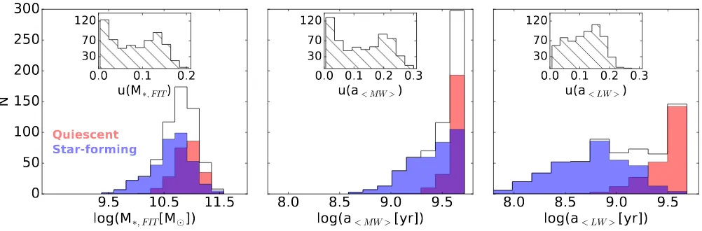
Figure3shows the distribution of the model-measured stellar masses (M∗,F IT, left panel), mean mass-weighted

ages2 _(a

<M W >, middle panel) and mean light-weighted

ages2 _(a

<LW >, right panel) of the LEGA-C sample,

along with the distribution of uncertainties for each pa-rameter. The distributions are separated into the quies-cent (red) and star-forming (blue) populations to show the differences in the distributions based on current SF activity (see Section 5). The galaxies in the LEGA-C sample span a broad range of ages: a<LW > can be as

young as 60 Myrs and as old as 4.8 Gyrs, and has a me-dian value of 1.2 Gyrs (see Figure 3). a<M W > ranges

from about 400 Myrs to about 5.2 Gyrs, with a median value of 3.8 Gyrs. However, most of these galaxies are old, with about 60% being older than 3 Gyrs. The

M∗,F IT of the galaxies ranges from ∼ 2×109M to

∼4×1011_M

, with a median value of about 6×1010M.

The formal age and mass uncertainties lie in the ranges 1-60% and 1-40%, respectively. As stated in Section

3.3, these uncertainties do not include systematic errors.

4.2. Sample SFHs

Figure 4 shows the spectra of a sample of LEGA-C galaxies (in a<M W > order) along with the

best-fitting model spectra as described by Equation 1 using the optimal parameter values from emcee. The weight

9.5

10.5 11.5

log(M

[M

])

0

50

100

150

200

250

300

N

Quiescent

Star-forming

8.0

8.5

9.0

9.5

log(a

[yr])

8.0

8.5

9.0

9.5

log(a

[yr])

0.0

0.1

0.2

u(M

)

30

70

120

0.0 0.1 0.2 0.3

u(a

)

30

70

120

0.0 0.1 0.2 0.3

u(a

)

30

70

120

Figure 3. Distributions of M∗,F IT(left), a<M W >(middle) and a<LW >(right) of the LEGA-C sample. The quiescent and

star-forming populations (as defined in Section5.1) are shown in red and blue, respectively. The distribution of the uncertainties for each parameter are shown at the top of each figure.

factors, mi, represent the star formation histories of

these galaxies (shown on the bottom-right of each fig-ure). The resultant normalised χ2_{, dust reddening}

val-ues (E(B−V)i), stellar masses (M∗,F IT), luminosities

(LF IT) and mean mass-weighted ages (a<M W >) from

the model are shown in red. The sample was selected to display the wide range of SFHs recovered.

The reconstructed SFHs reveal that although most galaxies at z ∼ 1 have a<M W >> 3 Gyrs, the sample

spans a wide range of histories. For the older massive galaxies, the oldest template (stars in the age range ∼3-7 Gyrs) contributes to the majority of their mass. Some of these galaxies only contain the oldest stars and have since been quiescent, i.e. for the past ∼ 3 Gyrs (see the SFHs of 108361, 211736 and 130052 in Figure 4). However, some galaxies were quiescent for several Gyrs and then had a renewed period of growth, either due to SF rejuvenation, or merging with a younger population. A merger could result in either an integration of the younger population with no further activity, or trigger bursts of star formation. This young population of stars accounts for ∼10 % of the mass of these galaxies (e.g. 206042, 131869 and 131393 in Figure4). We will explore the frequency of such rejuvenation events in more detail in a follow-up study.

4.3. General Trends

Figure5(a) presents the distribution of EW(Hδ) as a function of the Dn4000 break colour-coded by the time

after which the final 10% of stars were formed (a10, left

panel), a<LW > (middle panel) 3 and a<M W > (right

panel), estimated from the model. The EW(Hδ)-Dn4000

distribution is analysed in depth inWu et al.(2018). As expected, for all three age parameters, galaxies generally evolve from the upper-left region (high EW(Hδ) and low Dn4000) to the lower-right region (low EW(Hδ) and high

Dn4000) as they age. a10 and a<LW > are more

corre-lated with each other than a<M W > because they track

young stars; they also have smoother transitions in the EW(Hδ)-Dn4000 plane because those features primarily

track recent SF activity (_.1 Gyr). Figure5(b) shows the rest-frame U-V colour as a function of restframe V-J colour-coded by the same 3 age parameters as above. Once again, expected trends are seen: a10, a<LW >and

a<M W >correlate with the restframe colours as U-V and

V-J primarily reflect recent star formation (∼ 1 Gyr). There is a notable population of old galaxies (a<M W >

>3.5 Gyrs) with relatively blue colours, which indicates that these galaxies have extended SFHs.

To demonstrate the validity of the old galaxies

(a<M W > > 3.5 Gyrs) in the young region of the

EW(Hδ)-Dn4000 plane, i.e. galaxies in red in Figure

5’s right panel, with Dn4000 < 1.3 and EW(Hδ) > 2,

we refer to their SFHs. These galaxies formed most of their stars early on, but also have significant recent star formation. While some seem to have been quiescent at some point in their history before they were pos-sibly rejuvenated or merged with another galaxy (e.g. 206042 in Figure 4), others formed stars throughout their history (e.g. 210003 in Figure 4). Moreover, the

20

10

0

10

20

30

Flu

x [

10

−

19

er

g

s

−

1

cm

−

2

Å

−

1

]

ID: 96312

log(M∗

[M¯]) = 9.5

χ2

= 1.45

z = 0.72

log(L

[L¯]) = 10.7

E(B-V)

= 2.39

a

= 0.70

E(B-V)

= 0.01

Obs. Spectrum

Model

0

50

100

Flu

x [

10

−

19

er

g

s

−

1

cm

−

2

Å

−

1

]

ID: 116791

log(M∗

[M¯]) = 10.3

χ2

= 3.30

z = 0.66

log(L

[L¯]) = 11.7

E(B-V)

= 0.39

a

= 0.81

E(B-V)

= 0.09

Obs. Spectrum

Model

3800

4000

4200

4400

4600

4800

Rest-frame Wavelength [

Å

]

0

50

100

Flu

x [

10

−

19

er

g

s

−

1

cm

−

2

Å

−

1

]

ID: 111932

log(M∗

[M¯]) = 10.0

χ2

= 2.46

z = 0.63

log(L

[L¯]) = 11.3

E(B-V)

= 0.23

a

= 1.08

E(B-V)

= 0.10

Obs. Spectrum

Model

0

2

4

6

8

Age of Universe [Gyr]

0

10

20

SF

R

[M

/yr

]

0

2

4

6

8

Age of Universe [Gyr]

0

50

100

150

SF

R

[M

/yr

]

0

2

4

6

8

Age of Universe [Gyr]

0

50

100

150

SF

R

[M

/yr

]

40

20

0

20

40

60

Flu

x [

10

−

19

er

g

s

−

1

cm

−

2

Å

−

1

]

ID: 110967

log(M∗

[M¯]) = 10.8

χ2

= 2.47

z = 0.90

log(L

[L¯]) = 11.1

E(B-V)

= 0.28

a

= 2.18

E(B-V)

= 0.09

Obs. Spectrum

Model

0

20

40

60

80

Flu

x [

10

−

19

er

g

s

−

1

cm

−

2

Å

−

1

]

ID: 130052

log(M∗

[M¯]) = 11.0

χ2

= 1.86

z = 0.60

log(L

[L¯]) = 11.0

E(B-V)

= 2.04

a

= 3.92

E(B-V)

= 0.10

Obs. Spectrum

Model

3800

4000

4200

4400

4600

4800

Rest-frame Wavelength [

Å

]

0

20

40

60

Flu

x [

10

−

19

er

g

s

−

1

cm

−

2

Å

−

1

]

ID: 210003

log(M∗

[M¯]) = 10.6

χ2

= 2.84

z = 0.74

log(L

[L¯]) = 11.5

E(B-V)

= 0.53

a

= 3.97

E(B-V)

= 0.01

Obs. Spectrum

Model

0

2

4

6

8

Age of Universe [Gyr]

0

100

200

SF

R

[M

/yr

]

0

2

4

6

8

Age of Universe [Gyr]

0

50

100

SF

R

[M

/yr

]

0

2

4

6

8

Age of Universe [Gyr]

0

20

40

SF

R

[M

/yr

]

20

0

20

40

60

Flu

x [

10

−

19

er

g

s

−

1

cm

−

2

Å

−

1

]

ID: 131393

log(M∗

[M¯]) = 11.0

χ2

= 2.10

z = 0.73

log(L

[L¯]) = 11.0

E(B-V)

= 2.20

a

= 4.59

E(B-V)

= 0.08

Obs. Spectrum

Model

0

20

40

60

Flu

x [

10

−

19

er

g

s

−

1

cm

−

2

Å

−

1

]

ID: 206042

log(M∗

[M¯]) = 10.8

χ2

= 2.28

z = 0.61

log(L

[L¯]) = 10.9

E(B-V)

= 0.07

a

= 4.66

E(B-V)

= 0.13

Obs. Spectrum

Model

3800

4000

4200

4400

4600

4800

Rest-frame Wavelength [

Å

]

20

0

20

40

60

Flu

x [

10

−

19

er

g

s

−

1

cm

−

2

Å

−

1

]

ID: 139221

log(M∗

[M¯]) = 10.8

χ2

= 2.54

z = 0.70

log(L

[L¯]) = 11.0

E(B-V)

= 0.39

a

= 5.01

E(B-V)

= 0.05

Obs. Spectrum

Model

0

2

4

6

8

Age of Universe [Gyr]

0

20

40

60

SF

R

[M

/yr

]

0

2

4

6

8

Age of Universe [Gyr]

0

20

40

SF

R

[M

/yr

]

0

2

4

6

8

Age of Universe [Gyr]

0

20

40

SF

R

[M

/yr

]

20

0

20

40

Flu

x [

10

−

19

er

g

s

−

1

cm

−

2

Å

−

1

]

ID: 131869

log(M∗

[M¯]) = 10.7

χ2

= 1.29

z = 0.73

log(L

[L¯]) = 10.7

E(B-V)

= 2.18

a

= 5.03

E(B-V)

= 0.06

Obs. Spectrum

Model

20

0

20

40

60

Flu

x [

10

−

19

er

g

s

−

1

cm

−

2

Å

−

1

]

ID: 108361

log(M∗

[M¯]) = 10.9

χ2

= 1.72

z = 0.62

log(L

[L¯]) = 10.8

E(B-V)

= 0.03

a

= 5.13

E(B-V)

= 0.12

Obs. Spectrum

Model

3800

4000

4200

4400

4600

4800

Rest-frame Wavelength [

Å

]

20

0

20

40

60

Flu

x [

10

−

19

er

g

s

−

1

cm

−

2

Å

−

1

]

ID: 211736

log(M∗

[M¯]) = 11.1

χ2

= 2.54

z = 0.73

log(L

[L¯]) = 11.1

E(B-V)

= 0.53

a

= 5.13

E(B-V)

= 0.08

Obs. Spectrum

Model

0

2

4

6

8

Age of Universe [Gyr]

0

10

20

30

SF

R

[M

/yr

]

0

2

4

6

8

Age of Universe [Gyr]

0

20

40

SF

R

[M

/yr

]

0

2

4

6

8

Age of Universe [Gyr]

0

50

SF

R

[M

/yr

]

0.9

1.2

1.6

1.9

Dn4000

0

4

8

12

EW

H

δ

[

Å

]

0.9

1.2

1.6

1.9

Dn4000

0.9

1.2

Dn4000

1.6

1.9

0

1

2

3

4

5

a

[Gyr]

0

1

2

3

4

5

a

[Gyr]

0

1

2

3

4

5

a

[Gyr]

(a)

0.5

1.0

1.5

2.0

Rest-frame V-J

1.0

1.5

2.0

2.5

Rest-frame U-V

0.5

1.0

1.5

2.0

Rest-frame V-J

0.5

Rest-frame V-J

1.0

1.5

2.0

0

1

2

3

4

5

a

[Gyr]

0

1

2

3

4

5

a

[Gyr]

0

1

2

3

4

5

a

[Gyr]

(b)

Figure 5. EW(Hδ) versus Dn4000 (upper panel) and U-V colour versus V-J colour (lower panel) colour-coded by the time

after which the final 10% of stars were formed (left), the mean light-weighted age (middle), and the mean mass-weighted age (right). Typical error bars are indicated in grey.

presence of young and old populations can be seen in their spectra: they have clearly visible Balmer lines, characteristic of younger galaxies; but they also have H and K absorption lines of singly ionized Calcium with similar strengths, which is typical of older galaxies, in addition to the presence of the G-band (absorption lines of the CH molecule) around 4300 ˚A. As a test, we reran the fits of these galaxies excluding the 3 oldest templates and found that the spectra cannot be well fit.

There is also a population of galaxies that seem to con-tain only young stars (e.g. 111932 and 116791 in Figure

4), which would imply that these galaxies formed more than 90% of their mass recently (when the Universe was >6 Gyrs). To test if young populations are ‘outshin-ing’ the rest of these galaxies, i.e. if there are hidden populations of old stars, we reran the fits of these galax-ies allowing only the oldest template parameter to vary. We found that the contribution in mass of the old popu-lation can increase by∼5−10% before the normalised χ2 changes by more than 0.08 dex. The change in χ2

is mainly due to the continuum shape of the spectra. Therefore, these galaxies do not harbour significant populations of old stars that are concealed by the light of very young stars.

5. SFHS OF THE GALAXY POPULATION

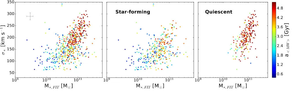
5.1. Correlations between Age, M∗,F ITandσ∗

Figure 6 shows a<M W > as a function of

stel-lar mass (M∗,F IT, left panel) and stellar velocity

dispersion (σ∗, right panel) colour-coded by

cur-rent SF activity, i.e. whether the galaxy is quiescent (log(sSFRU V+IR[Gyr−1]) < −1) or star-forming.

Se-lecting quiescent galaxies by their U-V and V-J col-ors would result in similar trends. a<M W > generally

correlates more strongly with M∗,F IT than σ∗.

How-ever, there is a σ∗ threshold above which galaxies are

almost exclusively old and quiescent: galaxies with σ∗> 200−250 km s−1 and a<M W >< 4 Gyrs are very

9.0

9.5

10.0

10.5

11.0

11.5

log(M∗

[M¯

])

8.6

8.8

9.0

9.2

9.4

9.6

9.8

log

(a

M

W

>

[y

r])

Star-forming

Quiescent

1.8

2.0

2.2

2.4

log(

σ

[km s

])

Figure 6. a<M W > as a function of M∗,F IT (left) andσ∗ (right). The star-forming and quiescent populations are indicated in blue and red, respectively, and typical error bars are indicated in grey. Galaxies withσ∗&200 km s−1 are almost exclusively old (>4Gyrs) and quiescent, which indicates thatσ∗ is a stronger predictor of age and SF activity.

10

₁₀

₁₀

M

[M

]

50

100

150

200

250

300

350

σ

[k

m

s

−

1

]

10

₁₀

₁₀

M

[M

]

Star-forming

10

₁₀

₁₀

M

[M

]

Quiescent

0.6

1.2

1.8

2.4

3.0

3.6

4.2

4.8

a

W

>

[G

yr

]

Figure 7. σ∗ versus M∗,F IT, colour-coded by a<M W >. The star-forming and quiescent populations are shown in the middle

and right panels, respectively. Typical error bars are indicated in grey. The clear separation between young and old galaxies atσ∗∼170 km s−1 shows a stronger correlation between a<M W > andσ∗ over M∗,F IT, which also depends on the current SF

activity.

high-mass galaxies (M∗,F IT&1011M) show a variety

of ages.

To further illustrate these trends, we show σ∗ as a

function of M∗,F IT colour-coded by a<M W > (left panel)

and divided by current SF activity (middle and right panels) in Figure7. There is a discernible separation be-tween old (>4 Gyrs) and young (<4 Gyrs) galaxies at a velocity dispersion of σ∗∼170 km s−1. Taken together

with the trends seen in Figure6, we can conclude that σ∗>250 km s−1is a sufficient requirement for having an

old age andσ∗∼170 km s−1 is a necessary requirement

for old age. This extends the properties of present-day

early-type galaxies, for which a correlation between ve-locity dispersion (and closely related quantities such as surface mass density and central mass density) and stel-lar age has been shown to be more fundamental than age trends with stellar mass (Kauffmann et al. 2003;van der Wel et al. 2009; Graves et al. 2009), to higher redshift. Our results also extend the widely reported correlation between velocity dispersion (as well as surface mass density and central mass density) and SF activity (e.g.,

1

2

3

4

5

6

7

Age of Universe [Gyr]

0.0

0.1

0.2

0.3

0.4

SF

R/

M

[G

yr

−

1

]

Mass [M

]

σ

<

120

σ

<

170

σ

<220

σ

1

2

3

4

5

6

7

Age of Universe [Gyr]

Star-forming

1

2

3

4

5

6

7

Age of Universe [Gyr]

Quiescent

1

2

3

4

6

Redshift

1

2

3

4

6

Redshift

1

2

3

4

6

Redshift

(a)

1

2

3

4

5

6

7

Age of Universe [Gyr]

0.0

0.1

0.2

0.3

0.4

SF

R/

M

[G

yr

−

1

]

Mass [M

]

log

M

<

.

10

.

log

M

<

.

10.8

log(M∗

<

log(M

1

2

3

4

5

6

7

Age of Universe [Gyr]

Star-forming

1

2

3

4

5

6

7

Age of Universe [Gyr]

Quiescent

1

2

3

4

6

Redshift

1

2

3

4

6

Redshift

1

2

3

4

6

Redshift

(b)

Figure 8. Ensemble-averaged SFHs of LEGA-C galaxies, normalised by stellar mass and separated into various σ∗ (top) and M∗,F IT, bins (bottom). The histories are divided into the star-forming and quiescent populations in the middle and right panels,

respectively. The stellar content in massive galaxies formed earlier and faster, regardless of current SF activity.

The scaling relation betweenσ∗ and black hole (BH)

mass implies that large BH mass is correlated with early SF and the ceasing thereof. Such a scenario is supported by the direct correlation between BH mass and SF ac-tivity (e.g., Terrazas et al. 2016) and the large fraction of radio AGN among galaxies with large velocity dis-persions both at low and high redshift (e.g., Best et al. 2005;Bariˇsi´c et al. 2017).

It is interesting to note that the correlation between a<M W > and σ∗ seen in Figure7 is significantly

weak-ened after dividing the population by current SF ac-tivity. Instead, for the star-forming population, galaxy age is better correlated with M∗,F IT (also seen in

Fig-ure 6). A straightforward interpretation is that when galaxies are growing rapidly through SF–that is, when they are located on or near the SF ‘Main Sequence’–then M∗mostly traces how long this main SF phase has lasted

so far. In other words, M∗simply traces the build-up of

the stellar population over time, while σ∗ is related to

the end of this main SF phase, i.e. to the regulation and cessation of SF, presumably through AGN feedback.

5.2. Evolution of the average SFHs

The average SFHs of galaxies, normalised by stellar mass, as a function of σ∗ and M∗,F IT are shown in

star-10

10

10

10

10

10

10

SF

R/

M

[G

yr

−

1

]

σ

<

115

_Star-forming

Quiescent

115

σ

<

160

1

2

3

4

5

6

7

8

Age of Universe [Gyr]

10

10

10

10

10

10

SF

R/

M

[G

yr

−

1

]

160

σ

<

205

1

2

3

4

5

6

7

8

Age of Universe [Gyr]

σ

205

Figure 9. SFHs of the LEGA-C sample (normalised by stellar mass) as a function of the age of the Universe separated into four

σ∗ bins indicated by the labels. The colours differentiate between the star-forming and quiescent populations at the observed redshift.

forming galaxies. These relations are used to determine whether z∼1 galaxies also show a downsizing trend in their SFHs, as many studies have pointed to using local galaxies. However, the SFHs seen at z ∼1 would not be resolved at z∼0.1, as the stellar populations would be too old.

On average, high-σ∗ galaxies (σ∗ ≥170 km s−1) had

higher SFRs at earlier epochs which started to de-cline rapidly, at a rate that increases with σ∗ and

stellar mass, when the Universe was ∼ 3 Gyrs old. Most galaxies with lower velocity dispersions (σ∗ <

170 km s−1) gradually build their stellar mass as the Uni-verse evolves; however, the SFR of a minority, i.e. the quiescent population, began to decline when the Uni-verse was∼5 Gyrs old. Higher-mass star-forming galax-ies (M∗,F IT≥1010.5M) have SFHs that are consistent

with constant star-formation with time, while the lower mass galaxies (M∗,F IT<1010.5) still have rising SFRs.

The star-forming population is still undergoing its main formation phase. The SFH trend is clear with M∗,F IT

and not σ∗ for the star-forming population, which

ex-tends from M∗,F IT being better correlated with SFHs

for star-forming galaxies as discussed in Section5.1(see Figure6 and7).

Figure 8 reveals that, on average, most galaxies in the sample were forming stars quite early on;

how-ever, the SFRs were systematically higher and the even-tual decline systematically more rapid with increasing

σ∗ (M∗,F IT for the star-forming population). This is

clear evidence for the top-down scenario; where galaxies downsize in their star formation with time (more mas-sive galaxies have older stars). This is seen in the overall population, and more strongly so in the quiescent pop-ulation. While this result is in alignment with previous studies for the local universe (e.g. Juneau et al. 2005;

Thomas et al. 2005;Tojeiro et al. 2009;McDermid et al. 2015;Ibarra-Medel et al. 2016), our work establishes this trend atz∼1 (half the current age of the Universe) us-ing spectroscopy.

5.3. The variety of SFHs

In Figure 9, we show all the stellar mass normalised SFHs in the LEGA-C sample, separated into four veloc-ity dispersion bins and divided into the quiescent and star-forming population (at the observed redshift) as de-fined in Section5.1. This reveals the large scatter in the SFHs at fixed mass, in addition to discerning the differ-ences in the histories based on the current star-formation activity of the galaxies.

grow in SFR, which peaked at later epochs. The qui-escent population has consistently higher SFRs at early epochs, whereas its star-forming counterpart has higher SFRs at later epochs. This indicates that star-forming galaxies aggregate their mass slower than the quiescent population. The dominance of the quiescent population increases from low to high-mass galaxies, and vice versa for the star-forming population.

The SFRs of low mass galaxies (σ∗ < 115 km s−1)

have been gradually increasing, with large scatter at all epochs. These galaxies are currently undergoing the main stages of their star formation. Note that the low-est dispersion bin suffers from incompleteness, due to the survey sample selection approach. K-band quiescent galaxies are fainter than equally massive star-forming galaxies which causes an under-representation in the LEGA-C sample. However, it is well known that low-mass star-forming galaxies outnumber quiescent galaxies of the same mass; therefore, the SFHs in Figure9 can be considered as illustrative.

The quiescent and star-forming populations are more evenly distributed (in number and variation of SFHs) in the intermediate-σ∗ regime (between

160 and 205 km s−1_{) while the high-σ}

∗ population

(σ∗ ≥ 205 km s−1) is dominated by quiescent galaxies.

The disparity between the SFHs of the quiescent and star-forming populations in the high-σ∗ regime

indi-cates that galaxies ‘remember’ their past. There is a strong coherence among the SFHs of quiescent and star-forming galaxies, respectively. This behaviour extends to the peak of cosmic SF activity at z ∼2-3. This im-plies that SF activity at the moment of observation is strongly correlated with the SF activity∼3 Gyrs prior. The results of this work indicate that many evolutionary paths can lead to galaxies at a given velocity dispersion. This illustrates the difficulty of connecting progenitor and descendant populations at different cosmic epochs.

5.4. Comparisons to Literature Measurements

As stated in Section 5.2, the deconstructed SFHs in this study support the galaxy downsizing scenario which has long been studied (see Section1). Leitner(2012)’s finding that star-forming galaxies formed only ∼15 % of their mass beforez= 1-2 (mass dependent), suggest-ing that present-day star-formsuggest-ing galaxies are not the descendants of massive star-forming galaxies at z > 2, is in line with our results since the peak in star formation occurs afterz <1.5 for almost all star-forming galaxies in the LEGA-C sample.

Intermediate-redshift stellar population studies are sparse, due to the high S/N required to undertake such studies (see Section 1). Pertaining to this work, there

are a few studies we can draw comparisons from, viz.

Choi et al. (2014) and Gallazzi et al. (2014). Mea-surements by Choi et al. (2014) and Gallazzi et al.

(2014) indicating that passive galaxies have ages con-sistent with mostly passive evolution are also in align-ment with this study as the reconstructed SFHs indicate that galaxies stay quiescent, barring some histories that showed low-level star formation after quiescence. Gal-lazzi et al.(2014) reported an average lighted-weighted age of∼5 Gyrs for a 4×1010_M

galaxy, consistent with

our value of 4.8 Gyrs, for a galaxy of the same mass.

Diemer et al.(2017) testedGladders et al.(2013)’s hy-pothesis that the SFHs of individual galaxies are charac-terised by a log-normal function in time, which implies a slow decline in SFRs rather than rapid quenching. They did this by comparing the log-normal parameter space of total stellar mass, peak time, and full width at half max-imum of simulated galaxies from Illustris (Vogelsberger et al. 2014) andGladders et al. (2013), as well as Paci-fici et al.(2016)’s derived SFHs of a sample of quiescent galaxies using a large library of computed theoretical SFHs. They found good agreement for all three stud-ies, however, Illustris predicted more extended SFHs on average. LEGA-C galaxies support the slow-quenching picture of galaxy evolution asGladders et al.(2013) have suggested, with a rate of decline that is mass dependent as we have seen. More comparisons will be performed in later papers.

6. SUMMARY

We have reconstructed the SFHs of galaxies in the current LEGA-C sample, which contains 678 primary sample galaxies with S/N∼20 ˚A−1_{in the redshift range}

0.6< z <1. We have done this by implementing an al-gorithm to fit flexible SFHs to the full spectrum, using

FSPS andemcee. The galaxy spectra were fit to a

lin-ear combination of a defined set of 12 CSPs, with solar metallicity and constant star formation within the time interval of the templates. In 90% of the cases the al-gorithm produced good fits based on the normalisedχ2

values. We found a wide variety of SFHs, although 60% of the galaxies have a<M W >> 3 Gyrs by the time we

observe them (Figures3and4). However, we note that age estimates from spectral fits experience increasing de-generacy of spectral features as the stellar populations age. Most of the old galaxies (a<M W >& 3 Gyrs) had

formed throughout the galaxies’ histories. The median a<LW >, a<M W > and M∗,F IT were found to be 1.2 Gyrs,

3.8 Gyrs and 1010.8_M

, respectively.

The main objective of this work was to investigate how our reconstructed SFHs behave as a function of stel-lar mass, stelstel-lar velocity dispersion and star-formation (SF) activity, as well as the variation they show at fixed velocity dispersion. We found that galaxies at z ∼ 1 have similar trends in their SFHs compared to local galaxies, i.e. the stellar content in massive galax-ies formed earlier and faster (Figure8). This top-down scenario is a known trend from fossil record inferences using SDSS spectra; however, in this study, it is shown forz∼1 galaxies for the first time. We found that the scatter between the quiescent and star-forming popula-tions increases towards lower redshift (Figure9), which indicates that current SF activity is strongly correlated with past SF activity. High-dispersion quiescent galax-ies had their star formation peak early, >9.5 Gyrs ago, and exhibit decreasing SFRs throughout the rest of their history, for the most part. We found that the lowest dis-persion galaxies in our sample are undergoing the main stage of their star formation as we observe them (7 Gyrs ago).

The results of the spectral fits were used to mea-sure a number of galaxy properties, viz. ages (a<LW >,

a<M W >, a<M W >, etc.) and stellar mass, in order

to test the model by investigating how these properties relate to one another as well as other properties mea-sured from the galaxy spectra, e.g. velocity dispersion, Hδ, Dn4000, etc. We showed that galaxies evolve from

the top-left to the bottom-right of the EW(Hδ)-Dn4000

plane as they age, as would be expected (Figure5). Recovering the full SFHs of intermediate-redshift galaxies opens up a multitude of avenues of research. In this work we have shown the clear differences between the SFHs of quiescent and star-forming galaxies and how these SFHs are scattered at fixed velocity disper-sion. We have also shown that velocity dispersion is a better indicator of the age and current SF activity of galaxies as a whole than stellar mass, while stellar mass is a better indicator of the age of star-forming galaxies (Figure 6 and 7). In future studies, we will use the reconstructed SFHs to constrain the quenching speed and rate, as well as investigate the relationship between galactic structure and SFHs. These constraints will be-come valuable for future surveys like JWST that will be investigating the properties of galaxies beyond z ∼ 2, and will need z ∼1 measurements as a benchmark to connect those populations to the local Universe.

7. ACKNOWLEDGEMENTS

Based on observations made with ESO Telescopes at the La Silla Paranal Observatory under programme ID 194-A.2005 (The LEGA-C Public Spectroscopy Survey). PC gratefully acknowledge financial support through a DAAD-Stipendium. This project has received funding from the European Research Council (ERC) under the European Union’s Horizon 2020 research and innovation programme (grant agreement No. 683184). KN and CS acknowledge support from the Deutsche Forschungse-meinschaft (GZ: WE 4755/4-1). We gratefully acknowl-edge the NWO Spinoza grant.

REFERENCES

Abramson, L. E., Gladders, M. D., Dressler, A., et al. 2016, ApJ, 832, 7

Bariˇsi´c, I., van der Wel, A., Bezanson, R., et al. 2017, ApJ, 847, 72

Barro, G., Faber, S. M., Koo, D. C., et al. 2017, ApJ, 840, 47

Belli, S., Newman, A. B., & Ellis, R. S. 2015, ApJ, 799, 206

Best, P. N., Kauffmann, G., Heckman, T. M., & Ivezi´c, ˇZ. 2005, MNRAS, 362, 9

Brammer, G. B., Whitaker, K. E., van Dokkum, P. G., et al. 2011, ApJ, 739, 24

Bruzual, G., & Charlot, S. 2003, MNRAS, 344, 1000

Calzetti, D., Armus, L., Bohlin, R. C., et al. 2000, ApJ, 533, 682

Cappellari, M., & Emsellem, E. 2004, PASP, 116, 138

Chabrier, G. 2003, PASP, 115, 763

Charlot, S., & Fall, S. M. 2000, ApJ, 539, 718

Choi, J., Conroy, C., Moustakas, J., et al. 2014, ApJ, 792,

95

Cid Fernandes, R., Asari, N. V., Sodr´e, L., et al. 2007,

MNRAS, 375, L16

Cid Fernandes, R., Mateus, A., Sodr´e, L., Stasi´nska, G., &

Gomes, J. M. 2005, MNRAS, 358, 363

Cimatti, A., Daddi, E., & Renzini, A. 2006, A&A, 453, L29

Conroy, C., & Gunn, J. E. 2010, ApJ, 712, 833

Conroy, C., Gunn, J. E., & White, M. 2009, ApJ, 699, 486

Diemer, B., Sparre, M., Abramson, L. E., & Torrey, P.

2017, ApJ, 839, 26

Foreman-Mackey, D., Hogg, D. W., Lang, D., & Goodman,

Foreman-Mackey, D., Sick, J., & Johnson, B. 2014, doi:10.5281/zenodo.12157.

https://doi.org/10.5281/zenodo.12157

Franx, M., van Dokkum, P. G., F¨orster Schreiber, N. M., et al. 2008, ApJ, 688, 770

Gallazzi, A., Bell, E. F., Zibetti, S., Brinchmann, J., & Kelson, D. D. 2014, ApJ, 788, 72

Gallazzi, A., Charlot, S., Brinchmann, J., White, S. D. M., & Tremonti, C. A. 2005, MNRAS, 362, 41

Girardi, L., Bressan, A., Bertelli, G., & Chiosi, C. 2000,

A&AS, 141, 371

Gladders, M. D., Oemler, A., Dressler, A., et al. 2013, ApJ,

770, 64

Goodman, J., & Weare, J. 2010, Communications in

Applied Mathematics and Computational Science, Vol. 5, No. 1, p. 65-80, 2010, 5, 65

Graves, G. J., Faber, S. M., & Schiavon, R. P. 2009, ApJ,

698, 1590

Heavens, A. F., Jimenez, R., & Lahav, O. 2000, MNRAS,

317, 965

Ibarra-Medel, H. J., S´anchez, S. F., Avila-Reese, V., et al.

2016, MNRAS, 463, 2799

Jørgensen, I., & Chiboucas, K. 2013, AJ, 145, 77

Jørgensen, I., Chiboucas, K., Berkson, E., et al. 2017, AJ, 154, 251

Juneau, S., Glazebrook, K., Crampton, D., et al. 2005, ApJL, 619, L135

Karim, A., Schinnerer, E., Mart´ınez-Sansigre, A., et al. 2011, ApJ, 730, 61

Kauffmann, G., Heckman, T. M., White, S. D. M., et al. 2003, MNRAS, 341, 54

Khostovan, A. A., Sobral, D., Mobasher, B., et al. 2015, MNRAS, 452, 3948

Koleva, M., Prugniel, P., Bouchard, A., & Wu, Y. 2009, A&A, 501, 1269

Kriek, M., van Dokkum, P. G., Labb´e, I., et al. 2009, ApJ, 700, 221

Kriek, M., Conroy, C., van Dokkum, P. G., et al. 2016, Nature, 540, 248

Kroupa, P., Aarseth, S., & Hurley, J. 2001, MNRAS, 321, 699

Leitner, S. N. 2012, ApJ, 745, 149

Madau, P., & Dickinson, M. 2014, ARA&A, 52, 415 Maraston, C., Str¨omb¨ack, G., Thomas, D., Wake, D. A., &

Nichol, R. C. 2009, MNRAS, 394, L107 Marigo, P., & Girardi, L. 2007, A&A, 469, 239

Marigo, P., Girardi, L., Bressan, A., et al. 2008, A&A, 482, 883

McDermid, R. M., Alatalo, K., Blitz, L., et al. 2015, MNRAS, 448, 3484

Mosleh, M., Tacchella, S., Renzini, A., et al. 2017, ApJ, 837, 2

Moustakas, J., Coil, A. L., Aird, J., et al. 2013, ApJ, 767, 50 Muzzin, A., Marchesini, D., Stefanon, M., et al. 2013a,

ApJ, 777, 18

—. 2013b, ApJS, 206, 8

Ocvirk, P., Pichon, C., Lan¸con, A., & Thi´ebaut, E. 2006, MNRAS, 365, 46

Onodera, M., Carollo, C. M., Renzini, A., et al. 2015, ApJ, 808, 161

Pacifici, C., Kassin, S. A., Weiner, B. J., et al. 2016, ApJ, 832, 79

Pozzetti, L., Bolzonella, M., Zucca, E., et al. 2010, A&A, 523, A13

S´anchez-Bl´azquez, P., Peletier, R. F., Jim´enez-Vicente, J., et al. 2006, MNRAS, 371, 703

Terrazas, B. A., Bell, E. F., Henriques, B. M. B., et al. 2016, ApJL, 830, L12

Thomas, D., Maraston, C., Bender, R., & Mendes de Oliveira, C. 2005, ApJ, 621, 673

Thomas, D., Maraston, C., Schawinski, K., Sarzi, M., & Silk, J. 2010, MNRAS, 404, 1775

Toft, S., Gallazzi, A., Zirm, A., et al. 2012, ApJ, 754, 3 Tojeiro, R., Heavens, A. F., Jimenez, R., & Panter, B.

2007, MNRAS, 381, 1252

Tojeiro, R., Wilkins, S., Heavens, A. F., Panter, B., & Jimenez, R. 2009, ApJS, 185, 1

Torrey, P., Wellons, S., Ma, C.-P., Hopkins, P. F., & Vogelsberger, M. 2017, MNRAS, 467, 4872

van de Sande, J., Kriek, M., Franx, M., et al. 2013, ApJ, 771, 85

van der Wel, A., Bell, E. F., van den Bosch, F. C., Gallazzi, A., & Rix, H.-W. 2009, ApJ, 698, 1232

van der Wel, A., Noeske, K., Bezanson, R., et al. 2016, ApJS, 223, 29

van Dokkum, P. G., & Brammer, G. 2010, ApJL, 718, L73 Vogelsberger, M., Genel, S., Springel, V., et al. 2014,

MNRAS, 444, 1518

Weisz, D. R., Dalcanton, J. J., Williams, B. F., et al. 2011, ApJ, 739, 5

Whitaker, K. E., van Dokkum, P. G., Brammer, G., & Franx, M. 2012, ApJL, 754, L29

Whitaker, K. E., van Dokkum, P. G., Brammer, G., et al. 2013, ApJL, 770, L39

Wilkinson, D. M., Maraston, C., Thomas, D., et al. 2015, MNRAS, 449, 328

Wu, P.-F., van der Wel, A., Gallazzi, A., et al. 2018, ArXiv e-prints, arXiv:1802.06799