Using Stochastic Gradient Markov
Chain Monte Carlo
Jack Baker, B.Sc.(Hons.), M.Res
Submitted for the degree of Doctor of Philosophy at Lancaster
University.
Markov chain Monte Carlo (MCMC), one of the most popular methods for inference on Bayesian models, scales poorly with dataset size. This is because it requires one or more calculations over the full dataset at each iteration. Stochastic gradient Markov chain Monte Carlo (SGMCMC) has become a popular MCMC method that aims to be more scalable at large datasets. It only requires a subset of the full data at each iteration. This thesis builds upon the SGMCMC literature by providing contributions that improve the efficiency of SGMCMC; providing software that improves its ease-of-use; and removes large biases in the method for an important class of model.
While SGMCMC has improved per-iteration computational cost over traditional MCMC, there have been empirical results suggesting that its overall computational cost (i.e. the cost for the algorithm to reach an arbitrary level of accuracy) is still O(N), whereN is the dataset size. In light of this, we show how control variates can be used to develop an SGMCMC algorithm ofO(1), subject to two one-off preprocessing steps which each require a single pass through the dataset.
While SGMCMC has gained significant popularity in the machine learning com-munity, uptake among the statistics community has been slower. We suggest this may
First, I’d like to thank the staff, students and management at the STOR-i Centre for Doctoral Training. This is such an enjoyable and stimulating atmosphere to do research in, and I hope the centre stays for a long while to come. I’d like to mention the directors of STOR-i especially: Jon Tawn, Kevin Glazebrook and Idris Eckley; whose tireless work has helped build such a great atmosphere at STOR-i. Thanks for giving me the opportunity to be part of this centre. I’d also like to thank the admin staff: Kim Wilson, Jennifer Bull and Wendy Shimmin; who make the department run so smoothly, and for putting up with me. I am very grateful for the financial support provided by EPSRC.
This work could not have happened without my supervisors: Paul Fearnhead, Christopher Nemeth and Emily Fox; thank you for all the time and effort you have put into this PhD project. They have taught me so much, both technical and not.
STOR-i obviously would not be the same without its students, and I’m really grateful to all of them, both past and present. I’ll remember the laughs, discussions and advice for a long time to come. There’s no doubt I’ll stay in touch with many of you. The CSML group members were also invaluable for their wealth of knowledge,
discussions and idea sharing.
I declare that the work in this thesis has been done by myself and has not been submitted elsewhere for the award of any other degree.
Jack Baker
Abstract I
Acknowledgements III
Declaration VI
Contents XI
List of Figures XV
List of Tables XVI
List of Abbreviations XVII
1 Introduction 1
1.1 Bayesian Inference . . . 1 1.2 Contributions and Thesis Outline . . . 3
2 Monte Carlo Methods and SGMCMC 7
2.1 Monte Carlo . . . 8 2.2 Markov Chain Monte Carlo . . . 9
2.2.1 Markov Chains and Stochastic Stability . . . 10
2.2.2 Gibbs Update . . . 14
2.2.3 Metropolis–Hastings Update . . . 15
2.3 Itˆo Processes for MCMC . . . 18
2.3.1 Markov Processes and Stochastic Stability . . . 18
2.3.2 Itˆo Processes and the Langevin Diffusion . . . 21
2.3.3 The Euler–Maruyama Method and ULA . . . 28
2.4 Stochastic Gradient Markov Chain Monte Carlo . . . 32
2.4.1 Background . . . 33
2.4.2 Comparison to Divide-and-Conquer MCMC . . . 40
3 Control Variates for Stochastic Gradient MCMC 54 3.1 Introduction . . . 54
3.2 Stochastic Gradient MCMC . . . 57
3.2.1 Stochastic Gradient Langevin Dynamics . . . 58
3.3 Control Variates for SGLD Efficiency . . . 59
3.3.1 Control Variates for SGMCMC . . . 61
3.3.2 Variance Reduction . . . 64
3.3.3 Computational Cost of SGLD-CV . . . 68
3.3.4 Setup Costs . . . 73
3.4 Post-processing Control Variates . . . 73
3.5 Experiments . . . 78
3.5.2 Probabilistic Matrix Factorisation . . . 81
3.5.3 Latent Dirichlet Allocation . . . 84
3.6 Discussion . . . 86
3.7 Acknowledgements . . . 87
4 sgmcmc: An R Package for Stochastic Gradient Markov Chain Monte Carlo 88 4.1 Introduction . . . 88
4.2 Introduction to MCMC and Available Software . . . 91
4.3 Stochastic Gradient MCMC . . . 95
4.3.1 Stochastic Gradient Langevin Dynamics . . . 96
4.3.2 Stochastic Gradient Hamiltonian Monte Carlo . . . 97
4.3.3 Stochastic Gradient Nos´e–Hoover Thermostat . . . 98
4.3.4 Stochastic Gradient MCMC with Control Variates . . . 99
4.4 Brief TensorFlow Introduction . . . 100
4.4.1 Declaring TensorFlow Tensors . . . 101
4.4.2 TensorFlow Operations . . . 102
4.5 Package Structure and Implementation . . . 105
4.5.1 Example Usage . . . 108
4.5.2 Example Usage: Storage Constraints . . . 114
4.6 Simulations . . . 120
4.6.1 Gaussian Mixture . . . 121
4.6.3 Bayesian Neural Network . . . 127
4.7 Discussion . . . 132
5 Large-Scale Stochastic Sampling from the Probability Simplex 134 5.1 Introduction . . . 134
5.2 Stochastic Gradient MCMC on the Probability Simplex . . . 137
5.2.1 Stochastic Gradient MCMC . . . 137
5.2.2 SGMCMC on the Probability Simplex . . . 139
5.2.3 SGRLD on Sparse Simplex Spaces . . . 140
5.3 The Stochastic Cox-Ingersoll-Ross Algorithm . . . 142
5.3.1 Adapting for Large Datasets . . . 143
5.3.2 SCIR on Sparse Data . . . 146
5.4 Theoretical Analysis . . . 147
5.5 Experiments . . . 149
5.5.1 Latent Dirichlet Allocation . . . 149
5.5.2 Bayesian Nonparametric Mixture Model . . . 150
5.6 Discussion . . . 153
6 Conclusions 154 6.1 Discussion . . . 154
6.2 Future Work . . . 156
A.2 Post-processing Proofs . . . 165
A.3 Experiments . . . 167
B Appendix to Chapter 5 172 B.1 Proofs . . . 172
B.2 Proofs of Lemmas . . . 179
B.3 CIR Parameter Choice . . . 180
B.4 Stochastic Slice Sampler for Dirichlet Processes . . . 180
B.5 Experiments . . . 185
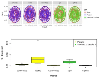
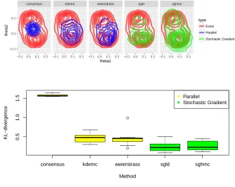
2.4.1 Comparison of method performance for multivariate-t distribution. Con-tour plots show empirical densities. Box plots show KL-divergence from the truth. . . 46 2.4.2 Comparison of method performance for Gaussian mixture. Contour
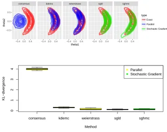
plots show empirical densities. Box plots show KL-divergence from the truth. . . 47 2.4.3 Comparison of method performance for warped Gaussian. Contour
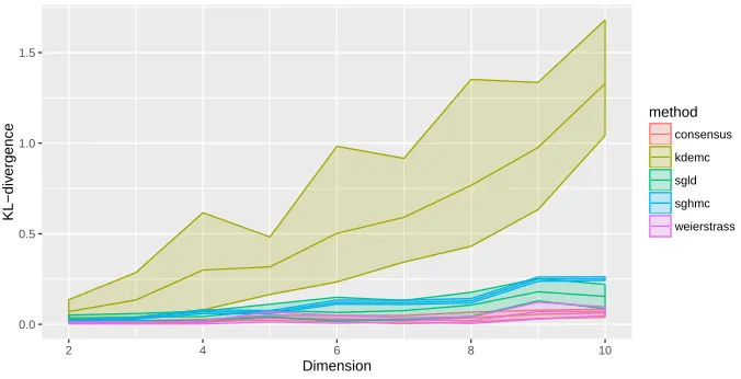
plots show empirical densities. Box plots show KL-divergence from the truth. . . 49 2.4.4 Comparison of method performance for Gaussian. Plot of KL-divergence
against dimension for each method. . . 51
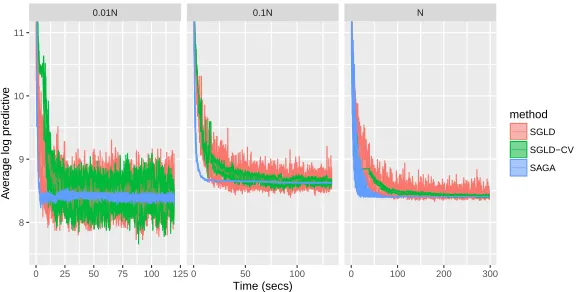
3.5.1 Log predictive density over a test set every 10 iterations of SGLD, SGLD-CV and SAGA fit to a logistic regression model as the proportion of data used is varied (as compared to the full dataset size N). . . 79
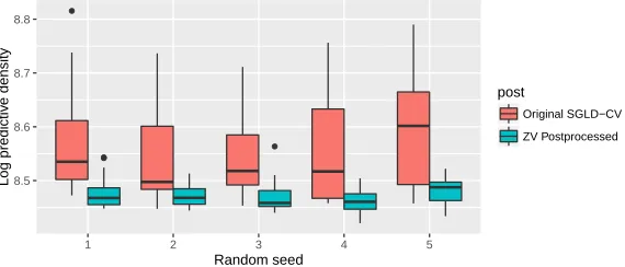
3.5.2 Plots of the log predictive density of an SGLD-CV chain when ZV post-processing is applied versus when it is not, over 5 random runs. Logistic regression model on the cover type dataset (Blackard and Dean, 1999). 80 3.5.3 Log predictive density over a test set of SGLD, SGLD-CV and SAGA
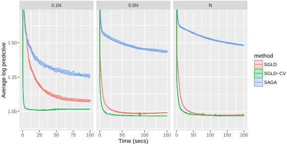
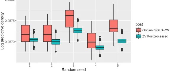
fit to a Bayesian probabilistic matrix factorisation model as the number of users is varied, averaged over 5 runs. We used the Movielens ml-100k dataset. . . 81 3.5.4 Plots of the log predictive density of an SGLD-CV chain when ZV
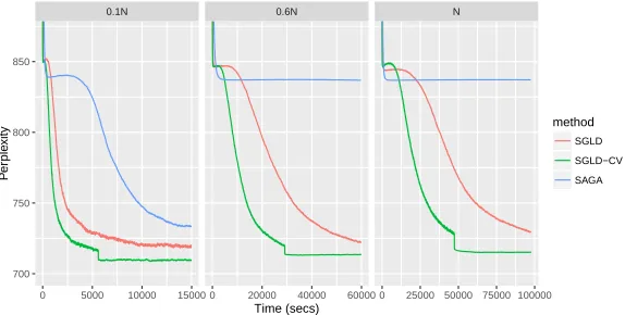
post-processing is applied versus when it is not, over 5 random runs. SGLD-CV algorithm applied to a Bayesian probabilistic matrix factorisation problem using the Movielens ml-100k dataset. . . 82 3.5.5 Perplexity of SGLD and SGLD-CV fit to an LDA model as the data
size N is varied, averaged over 5 runs. The dataset consists of scraped Wikipedia articles. . . 84
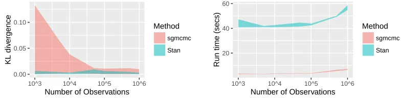
4.2.1 KL divergence (left) and run time (right) of the standard Stan algorithm and the sgldcv algorithm of the sgmcmc package when each are used to sample from data following a standard Normal distribution as the number of observations are increased. . . 93 4.5.1 Log loss on a test set for parameters simulated using the sgldcv
4.6.1 Plots of the approximate posterior for θ1 simulated using each of the
methods implemented by sgmcmc, compared with a full HMC run, treated as the truth, for the Gaussian mixture model (4.6.1). . . 124 4.6.2 Plots of the log loss of a test set for β0 and β simulated using each of
the methods implemented by sgmcmc. Logistic regression problem with the covertype dataset. . . 126 4.6.3 Plots of the log loss of a test set for θ simulated using each of the
methods implemented by sgmcmc. Bayesian neural network model with the MNIST dataset. . . 131
5.2.1 Boxplots of a 1000 iteration sample from SGRLD and SCIR fit to a sparse Dirichlet posterior, compared to 1000 exact independent samples. On the log scale. . . 141 5.3.1 Kolmogorov-Smirnov distance for SGRLD and SCIR at different
mini-batch sizes when used to sample from (a), a sparse Dirichlet posterior and (b) a dense Dirichlet posterior. . . 146 5.5.1 (a) plots the perplexity of SGRLD and SCIR when used to sample from
A.3.1 Log predictive density over a test set every 10 iterations of SGLD (with a decreasing stepsize scheme), SGLD-CV and SAGA fit to a logistic regression model as the data sizeN is varied. . . 169 A.3.2 Log predictive density over a test set of SGLD (with a decreasing
4.5.1 Outline of 6 main functions implemented in sgmcmc. . . 106 4.5.2 Outline of the key arguments required by the functions in Table 4.5.1. 107
A.3.1 Minibatch sizes for each of the experiments in 3.5 (they were fixed for SGLD, SGLD-CV and SAGA). . . 168 A.3.2 Tuned stepsizes for the Logistic regression experiment in Section 3.5.1. 168 A.3.3 Tuned stepsizes for the Bayesian probabilistic matrix factorisation
ex-periment in Section 3.5.2. . . 170 A.3.4 Tuned stepsizes for the Bayesian probabilistic matrix factorisation
ex-periment in Section 3.5.2. . . 171
B.5.1 Stepsizes for the synthetic experiment . . . 186 B.5.2 Hyperparameters for the LDA experiment . . . 187 B.5.3 Hyperparameters for the Bayesian nonparametric mixture experiment 187
MCMC Markov Chain Monte Carlo
SGMCMC Stochastic Gradient Markov Chain Monte Carlo a.s. Almost Surely
a.e. Almost Everywhere MH Metropolis–Hastings LD Langevin Diffusion
SDE Stochastic Differential Equation TV Total Variation
ULA Unadjusted Langevin Algorithm
MALA Metropolis–Adjusted Langevin Algorithm MSE Mean Square Error
RMSE Root Mean Square Error HMC Hamiltonian Monte Carlo
SGLD Stochastic Gradient Langevin Dynamics SGD Stochastic Gradient Descent
SGHMC Stochastic Gradient Hamiltonian Monte Carlo
PDP Piecewise Deterministic Process CIR Cox-Ingersoll-Ross Process
Introduction
Markov chain Monte Carlo (MCMC), one of the most popular methods for inference in Bayesian models, is known to scale poorly with dataset size. This has become a problem due to the growing complexity of practical models in both statistics and machine learning. This thesis provides contributions for stochastic gradient Markov chain Monte Carlo, a popular class of MCMC which aims to mitigate this problem.
In this chapter we set up the problem by providing a brief introduction to Bayesian inference and outlining the inherent scalability problems. This is elaborated on in Chapter 2, which provides a literature review of Monte Carlo methods and scalability. We then outline the contributions of this thesis, as well as the structure of the chapters.
1.1
Bayesian Inference
In most statistical and machine learning problems, interest is in an unknown parame-terθ. For simplicity, for now we suppose thatθ takes values inRd; but this is relaxed
in Chapter 2. Suppose relevant data is collected x = {xi}Ni=1, with xi ∈ Rd. Then Bayesian inference assumes that θ is a random variable, and aims to calculate the distribution of θ given this new information x, i.e. the distribution of θ|x. We refer to this distribution asπ. Treating θ as a random variable rather than a fixed quan-tity can alleviate overfitting, which is important for the complex models currently in popular use.
Suppose the dataxdepend on a random parameterθthrough the densitypi(θ) := p(xi|θ), here we assume that θ takes values in Rd. We assignθ a prior density p0(θ).
Then, the posterior density p(θ) := p(θ|x) (i.e. the density of π) is given by
p(θ) = QN
i=0pi(θ)
Z , Z =
Z
Rd
N Y
i=0
pi(θ)dθ, (1.1.1)
whereZ is referred to as the normalising constant.
IfZcan be calculated, thenp(θ) can be calculated analytically, giving a closed form expression detailingθ|x(though further integration would be required to obtain the distribution function itself). However, a fundamental problem in Bayesian inference is that the integration to find Z is rarely tractable. This means typically we only know the posterior up to the unnormalised density h(θ) := QNi=0pi(θ). MCMC gets around this issue by constructing an algorithm that will converge to sampling from π; while only needing to evaluate the unnormalised density h (for exact details see Section 2.2). Most quantities of interest can be written in the form Eπ[ψ(θ)]. This quantity can then be estimated using the MCMC sampleθm, m= 1, . . . , M by using the Monte Carlo estimate
Eπ[ψ(θ)]≈ 1 M
M X
m=1
In many modern statistics and machine learning problems, the dataset sizesN are very large. However, MCMC requires the calculation of h at each iteration. Since h is a product of N + 1 terms, this is an O(N) calculation and can cause MCMC to be prohibitively slow for large datasets. This has sparked interest in improving the computational efficiency of MCMC. One of the most popular methods for doing so is stochastic gradient MCMC (SGMCMC), which uses a subset of the data at each iteration of size n. This enables an algorithm to be implemented with O(n) calculations at each iteration. The main cost for the improved efficiency is that SGMCMC samples are no longer guaranteed to converge toπ.
1.2
Contributions and Thesis Outline
This thesis has focussed on developing three aspects of SGMCMC: efficiency, ease-of-use, and performance on an important class of problems. Contributions include: providing a detailed review of SGMCMC, including details of underlying theory and a comparison to an alternative popular class of scalable MCMC; establishing a frame-work for SGMCMC which provably improves its overall computational cost; develop-ing a software package for SGMCMC which enhances its ease of implementation; and improving the performance of SGMCMC when the method is used to sample from simplex spaces, an important class of problem.
Chapter 2: Monte Carlo Methods and Scalability
This Chapter provides a review of SGMCMC. The chapter first outlines standard MCMC methods. Then useful background material for SGMCMC is detailed, includ-ing continuous-time Markov processes and Itˆo processes. Important methodology in the SGMCMC literature is outlined based on the background material. Comparisons between SGMCMC and divide-and-conquer MCMC, an alternative popular class of scalable MCMC methods, are provided.
Chapter 3: Control Variates for Stochastic Gradient MCMC
This chapter is a journal contribution with co-authors Paul Fearnhead, Emily B. Fox and Christopher Nemeth. The manuscript has been accepted by the journal “Statistics and Computing.” The abstract of the publication is given below.
a different control variate technique, known as zero variance control variates, can be applied to SGMCMC algorithms for free. This post-processing step improves the in-ference of the algorithm by reducing the variance of the MCMC output. Zero variance control variates rely on the gradient of the log-posterior; we explore how the variance reduction is affected by replacing this with the noisy gradient estimate calculated by SGMCMC.
Chapter 4: sgmcmc: An R Package for Stochastic Gradient Markov Chain
Monte Carlo
This chapter is a journal contribution with co-authors Paul Fearnhead, Emily B. Fox and Christopher Nemeth. The manuscript has been accepted by the journal “Journal of Statistical Software.” The abstract of the publication is given below.
SGMCMC has become widely adopted in the machine learning literature, but less so in the statistics community. We believe this may be partly due to lack of software; this package aims to bridge this gap.
Chapter 5: Large-Scale Stochastic Sampling from the Probability Simplex
This chapter is conference proceedings appearing in “Advances in Neural Information Processing Systems” in 2018, with co-authors Paul Fearnhead, Emily B. Fox and Christopher Nemeth. The abstract of the publication is given below.
Monte Carlo Methods and
SGMCMC
Many statistical and machine learning problems can be reduced to the calculation of an expectation with respect to a probability distribution. The main problem that then needs to be overcome is that these expectations can rarely be calculated ana-lytically. Monte Carlo methods use the fact that these expectations can be simply approximated when the probability distribution can be simulated from. In Section 2.1, we explain the Monte Carlo procedure. While this simplifies the problem, often the underlying probability distribution is difficult to simulate from, especially in the Bayesian paradigm. In light of this, Section 2.2 details Markov chain Monte Carlo methods (MCMC), which can be used to simulate from a large class of probability dis-tributions. The most popular scalable MCMC methods, stochastic gradient Markov chain Monte Carlo (SGMCMC), are based on continuous-time Itˆo processes, so in Section 2.3.2 we provide an introduction to these processes, as well as the numerical
approximation procedure which forms the basis for many of these algorithms. Finally in Section 2.4 we detail SGMCMC methods, which form the basis for the rest of this thesis, and are some of the most popular scalable MCMC samplers. We also provide a comparison of some popular SGMCMC methods to a class of competitor algorithms known as divide-and-conquer MCMC. This forms the first contribution of this thesis. Monte Carlo is a large and varied topic, so only the topics necessary for this thesis are presented here. For a more thorough treatment of standard MCMC, please see Robert and Casella (2004); Meyn and Tweedie (1993a); for a more thorough treatment of Itˆo processes and their approximation we refer the reader to Øksendal (2003); Kloeden and Platen (1992); Khasminskii (2011).
2.1
Monte Carlo
Many statistical and machine learning problems can be reduced to the calculation of the expectation of a function. Let θ be a random variable taking values in some topological space Θ with distribution π (i.e. P(θ ∈ A) = π(A)). Denote the Borel σ-algebra for Θ by B(Θ). Note we use some simple measure-theoretic concepts (see e.g. Williams, 1991) to make notation clearer, and this allows us to avoid multiple definitions on different classes of Θ; but this thesis aims to be light on measure theory.
Most statistical quantities of interest can be reduced to
¯
ψ :=Eπ[ψ(θ)] = Z
Θ
ψ(θ)π(dθ), (2.1.1)
methods, such as quadrature, suffer from the curse of dimensionality. Monte Carlo methods get around this issue by assuming we can simulate from π. Let θ1, . . . , θM be a sequence of independent, identically distributed simulations from π. Then the Monte Carlo estimate of ¯ψ is defined by
ˆ ψM =
1 M
M X
m=1
ψ(θm). (2.1.2)
This estimate has a number of desirable statistical properties. The strong law of large numbers can be immediately applied to show that asM → ∞, ˆψM converges almost surely (a.s.) to ¯ψ, i.e.
ˆ ψM
a.s.
−−→ψ,¯ asM → ∞.
Similarly, supposeVar[ψ(θ)] =σ2 <∞, then the central limit theorem can be applied
to show that,
√
M( ˆψM −ψ)¯
D
−→N(0, σ2), asM → ∞ (2.1.3)
where−→D denotes convergence in distribution.
2.2
Markov Chain Monte Carlo
we introduce specific MCMC algorithms, we first need to introduce some results for Markov chains and stochastic stability.
2.2.1
Markov Chains and Stochastic Stability
Letθm,m= 1, . . . , M, be a discrete-time stochastic process taking values in Θ. Then this stochastic process is a Markov chain if it satisfies the Markov property; namely the future state θm+1 is independent of previous states given the value of the current
stateθm =ϑ. For notational convenience it is common to define a quantity known as the Markov kernelK : (Θ,B(Θ))→[0,1] as the following conditional probability
K(ϑ, A) =P(θm+1 ∈A|θm =ϑ).
Then the Markov property can be stated as follows
K(ϑm, A) = P(θm+1 ∈A|θm =ϑm) = P(θm+1 ∈A|θm =ϑm, . . . , θ1 =ϑ1).
We will also use the shorthand thatKm(ϑ, A) =K◦ · · · ◦K
| {z }
m
(ϑ, A); and that for some functionψ taking inputs in Θ, Kψ(ϑ) = RΘK(ϑ, dθ)ψ(θ)dθ.
Since we eventually wish to construct Markov chains that converge to the desired π, we need some way of assessing this. Before we can do this, we need some definitions. A Markov chain is defined to be stationary if the distribution ofθmdoes not depend on m, i.e. the Markov chain is drawn from a single distribution. An invariant distribution π of a Markov chain has the property that θm−1 ∼ π =⇒ θm ∼ π. A Markov chain with kernelK has invariant distributionπ if the following condition holds (Meyn and Tweedie, 1993a; Geyer, 2005) referred to as detailed balance or reversibility
Z
B
π(dϑ)K(ϑ, A) = Z
A
Now suppose we have a desired π, and wish to construct a Markov chain with kernelK that converges to sampling from π. Then we need to check two things: that the Markov chain converges to stationarity, that the stationary distribution of this Markov chain is uniquelyπ. If we know that the Markov chain leavesπinvariant, then there are two further properties that ensure this is the case: Harris recurrence and aperiodicity. If Harris recurrence holds then this ensures the invariant distribution is unique. A Markov chain is Harris recurrent if there exists a non-zero, σ-finite measure ϕ on B(Θ), such that for all for all A ∈ B(Θ), with ϕ(A) > 0; and for all ϑ ∈ Θ, a chain starting from ϑ will eventually reach A with probability one (Meyn and Tweedie, 1993a; Geyer, 2005). A Harris recurrent Markov chain is aperiodic if there does not exist an integerb >1, and disjoint subsetsB1, . . . Bb ∈ B(Θ) such that, for all i = 1, . . . , b we have ϕ(Bi)> 0 and K(ϑ, Bi) = 1, when ϑ ∈ Bj for j =i−1 modb (Meyn and Tweedie, 1993a; Geyer, 2005).
Once it is established that a Markov chain is Harris recurrent and aperiodic, then desirable properties similar to the results for Monte Carlo presented in the previous section can be established. Let θ1, . . . , θM be a Harris recurrent, aperiodic Markov chain. Let ˆψM be as defined in (2.1.2). Then
ˆ ψM
a.s.
−−→ψ,¯ asM → ∞, (2.2.1)
for any starting distribution λ. A central limit result for MCMC, similar to standard Monte Carlo, can also be derived (Robert and Casella, 2004; Geyer, 2005).
methods to the target π, so we will outline these results. First we need to describe the total variation metric, used to calculate the distance between two probability measures. A measure can be decomposed into its positive and negative parts for any setA ∈Θ asµ(A) =µ+(A)−µ−(A), where µ+(A), µ−(A) are positive measures with disjoint support. The total variation norm of some measure µ, can then be defined by
kµkT V =µ+(A) +µ−(A).
If the distribution defined by θm converges in total variation to π given any initial distributionλ, then it is said to be ergodic; i.e.
Z
λ(dϑ)KM(ϑ,·)−π
T V
M→∞
−−−−→0.
This property holds ifθmis Harris recurrent and aperiodic (Meyn and Tweedie, 1993a; Geyer, 2005).
Results on the convergence of SGMCMC methods require a stronger condition though, known as geometric ergodicity (Meyn and Tweedie, 1993a; Geyer, 2005). Geometric ergodicity bounds the non-asymptotic total variation distance. A Markov chain θm is said to be geometrically ergodic if there exists a function β : Θ → R+,
with β(θ)<∞ π-a.e.1, and a constant ρ <1, such that
kKm(ϑ,·)−πkT V ≤β(ϑ)ρm, ϑ ∈Θ.
Geometric ergodicity can be verified using a ‘drift condition,’ or Lyapunov–Foster condition. This relies on the existence of a norm-like function V and a petite set
1Given a measureπonB(Θ), a property holds almost everywhere (π-a.e.) if there existsN ∈ B(Θ)
C. The norm-like function V has the properties that V(θ) ≥ 1 and V(θ) → ∞ as kθk → ∞. It plays a similar role to Lyapunov functions, introduced in Section 2.3;
which are useful for deriving convergence results for SGMCMC. A set C is petite if there exists a probability distribution a, defined over N; a constant δ > 0; and a probability measure Q, defined overθ; such that
∞
X
m=0
a(m)Km(ϑ, A)≥δQ(A), ϑ ∈Θ.
To show a Markov chain is geometrically ergodic we then need a norm-like function V, a petite set C and constants λ <1 and b <∞ such that
KV(ϑ)≤λV(ϑ) +b1C, ϑ∈Θ.
This is known as a geometric drift condition. Drift conditions also exist to ensure a variety of properties of the Markov chain, including Harris recurrence (see e.g. Meyn and Tweedie, 1992)
Geometric ergodicity can be used to ensure a central limit theorem (CLT) holds for the Markov chain, similar to the CLT for Monte Carlo (2.1.3). In particular, let ψ : Θ → R be some test function of interest, and assume that Eπ[(ψ(θ))2+δ] < ∞ for some δ >0. If a Markov chain θm with stationary distributionπ is geometrically ergodic, as usual define ¯ψ =Eπ[ψ(θ)], then
1 √
M M X
m=1
ψ(θm)−ψ¯
D
−→N(0, σ2), as M → ∞; (2.2.2)
2.2.2
Gibbs Update
Now that we have covered the Markov chain background required, we introduce some popular transition kernels K used to sample from a given π. The Gibbs sampler (Geman and Geman, 1984) is a particularly simple Markov kernel used for multiple parameter problems. Suppose we are able to divide a multivariateθ ∈Θ into compo-nentsj = 1, . . . , d, such thatθ = (θ1, . . . , θd). For example, if we have interest in the targetπ(µ, σ) = N(µ, σI), whereIis the identity matrix; then we might divideθ into two parametersθ = (µ∈R2, σ∈
R) (notice that θj need not necessarily be a scalar). Then for each component of the partition, j, the Gibbs sampler updates θj as-suming the rest θ−j = (θ1, . . . , θj−1, θj+1, . . . , θd) is fixed at the previous state ϑ. To do this it uses the conditional distribution of the desired target,π(· |θ−j =ϑ−j). For each component j, the Gibbs update kernel can be defined as follows
Kj(ϑ, A) = 1ϑ−j∈A−jπ(Aj|θ−j =ϑ−j),
whereA= (A1, . . . , Ad) and A−j = (A1, . . . , Aj−1, Aj+1, . . . , Ad).
To show this update leaves π invariant we can use properties of the conditional expectation (Geyer, 2005). First notice that Kj(ϑ, A) = 1ϑ−j∈A−jE[1θj∈Aj|θ−j =
ϑ−j] =E[1ϑj∈A−j1θj∈Aj|θ−j =ϑ−j], so that by the law of total expectation
Z
Θ
π(dϑ)K(ϑ|A) =E[E[1ϑ−j∈A−j1θj∈Aj|θ−j =ϑ−j]] =π(A)
each iteration, but in any order; or to pick a j with probability 1/d, and update using kernelKj. Additional conditions on the state space Θ and K ensure the Gibbs sampler is Harris recurrent (see Meyn and Tweedie, 1993a; Robert and Casella, 2004; Geyer, 2005, for details). A Harris recurrent Gibbs sampler is always aperiodic.
Gibbs updates require no user tuning, and can make large moves since updating component j does not depend on θj, just θ−j. However, the Gibbs sampler can mix slowly when components are highly dependent. Another major disadvantage is that it requires the calculation of the conditional distributionsπ(·|θ−j). While there are many important machine learning and statistical problems where this is possible, there are also many problems where it is not.
2.2.3
Metropolis–Hastings Update
Commonly the only information we have aboutπ is an unnormalised density. We say a function h : Θ → R is an unnormalised density if it has the following properties: h is nonnegative; and 0 < R
Θh(θ)dµ < ∞, where µ is defined to be the Lebesgue
measure.
An important example where the only information we have about π is its unnor-malised density is in Bayesian inference. Suppose we have data x = {xi}Ni=1 which
depends on a parameter θ through the density pi(θ) := p(xi|θ). We assign θ a prior density p0(θ). Then, defining the Lebesgue measure by µ, the posterior density p(θ)
is given by
p(θ) = QN
i=0pi(θ)
Z , Z =
Z
Θ
N Y
i=0
where Z is referred to as the normalising constant. A fundamental problem in Bayesian inference is that the integration to find Z is rarely tractable. This means typically we only know the posterior up to the unnormalised densityh(θ) =QNi=0pi(θ). The Metropolis–Hastings algorithm aims to get around this issue by defining a Markov chain that converges to sampling from π and only relies on being able to evaluate h, where h is an unnormalised density of π. The Metropolis–Hastings algo-rithm (MH) was first developed by Metropolis et al. (1953), with an important later development by Hastings (1970), as well as Green (1995).
The main idea behind MH is to find a distribution Q, that is easy to simulate from, referred to as a proposal distribution. Then to correct simulations from this distribution so that the resulting process θm converges to sampling from π. More formally, suppose the Markov chain is currently at a stateθ. A proposal distribution, Q(·|θ), is used in order to simulate a new proposal state θ0 given the current state θ. Suppose this proposal distribution admits a density q(θ0|θ) with respect to the Lebesgue measure µ; then the Metropolis–Hastings algorithm proceeds as follows: a candidate state θ0 is simulated from Q, this candidate state is then accepted with probability
α(θ0, θ) = 1∧ h(θ
0)q(θ|θ0)
h(θ)q(θ0|θ),
wherec1∧c2 denotes the minimum between numbersc1 andc2. If the candidate value
these constants cancel in the ratio of terms; this is why any unnormalised density of π can be used to implement this algorithm.
To check the MH algorithm leaves π invariant we will show that the MH kernel satisfies detailed balance. Because the accept-reject step can lead to the algorithm staying in the current state, the Markov kernel for the MH algorithm is in the form of a sum
K(θ, A) =
1− Z
A
q(θ0|θ)α(θ, θ0)µ(dθ0)
1(θ ∈A) + Z
A
q(θ0|θ)α(θ, θ0)µ(dθ0),
where 1(θ ∈ A) is 1 if θ ∈ A and 0 otherwise. We demonstrate detailed balance informally by showing p(θ)K(θ, dθ0) = p(θ0)K(θ0, dθ), for a more formal proof see Robert and Casella (2004). We make use of the following identities, which can easily be checked: p(θ)q(θ0|θ)α(θ, θ0) =p(θ0)q(θ|θ0)α(θ0, θ), and p(θ)δ
θ0(θ) =p(θ0)δθ(θ0). We can apply these identities to check detailed balance as follows
p(dθ)K(θ, dθ0) = p(dθ) [1−q(θ0|θ)α(θ, θ0)]δθ0(θ) +p(dθ)q(θ0|θ)α(θ, θ0) =p(dθ0) [1−q(θ|θ0)α(θ0, θ)]δ
θ(θ0) +p(dθ0)q(θ|θ0)α(θ0, θ) =p(dθ0)K(θ0, dθ).
Metropolis–Hastings update has acceptance probability 1 (Robert and Casella, 2004; Geyer, 2005).
If our proposal and state space ensure Harris recurrence and aperiodicity then the MH sample is guaranteed to satisfy the strong law of large numbers result (2.2.1). For practical purposes though, we only simulate from our chain for a finite amount of time, so to ensure good properties of the chain we need to choose a good proposal distribution. The MSE of the chain tends to be controlled by the autocovariance, so the best proposals lead to chains with low autocovariance. In the next section we discuss how to construct efficient proposals for the MH algorithm using continuous-time Markov processes.
2.3
Itˆ
o Processes for MCMC
Many MCMC algorithms, including SGMCMC, rely on the theory of continuous-time Markov processes, in particular Itˆo diffusions. In this section we review results about these processes, so that the necessary grounding has been discussed when we summarise SGMCMC.
2.3.1
Markov Processes and Stochastic Stability
2011) if, for all A∈ B(Rd), 0≤s ≤t,
P(θt∈A| Fs) =P(θt ∈A|θs). (2.3.1) Our interest will be in Markov processes that are time-homogeneous, meaningP(θt ∈ A|θs) = P(θt−s ∈ A|θ0). This allows us to use the following shorthand for the
transition probabilityP(θt∈A|θ0 =ϑ) = Kt(ϑ, A). Provided it exists, we can define the transition densitypt(ϕ|ϑ) of the Markov process by
Kt(ϑ, A) = Z
A
pt(ϕ|ϑ)dϕ.
As in discrete-time Markov chains, we are often interested in the behaviour of a test function ψ under the dynamics of θt. We define
Ktψ(ϑ) = Z
Kt(ϑ, dy)ψ(y).
This allows us to define the operator known as thegenerator A (see e.g. Khasminskii, 2011) of the process, applied to a functionψ (provided the limit exists), as
Aψ(ϑ) = lim t→+0
Ktψ(ϑ)−ψ(ϑ)
t .
It can be shown the generator fully defines the Markov process (see e.g. Khasminskii, 2011). It can be visualised as describing the infinitesimal evolution of the process.
Similar to discrete-time Markov chains, we are interested in convergence of θt to a stationary distribution π. Necessary conditions for θt to be stationary are: for A, B ∈ B(Rd), and for all h > 0, the events {θ
t ∈ A} and {θt ∈ A, θt+h ∈ B} are independent of t; that the initial distribution π0 is invariant (see e.g. Khasminskii,
2011); i.e. for every s >0,
π0(A) =
Z
The idea behind finding stationary distributions for Markov processes is to again derive a law of large numbers forθt. Specifically, given some test functionψ, we desire results of the form
1 T
Z T
0
ψ(θt)dt a.s.
−−→ψ,¯ T → ∞.
Similarly to the law of large numbers for Markov chains, this relies on existence and uniqueness of the stationary solution to the chain (see e.g. Khasminskii, 2011). Conditions for this to be the case are investigated for Markov processes in Meyn and Tweedie (1993b,c). Similarly to Markov chains, a sufficient condition for the existence and uniqueness of a stationary solutionπis Harris recurrence. The definition of Harris recurrence is the same as for Markov chains, i.e. there exists a measureν on Θ such that the probability a chain θt ever hits a set A is one, for all ϑ ∈Θ and A ∈ B(Θ) with ν(A) > 0 (Meyn and Tweedie, 1993c). Moreover, if a Markov process θt is Harris recurrent and time points t1, . . . tM can be chosen such that the Markov chain
θtm is also Harris recurrent, then θtis ergodic, i.e. limt→∞kKt(ϑ,·)−πkT V = 0 for all ϑ∈Θ.
In Meyn and Tweedie (1993c), sufficient conditions are derived for desirable Markov process properties, such as Harris recurrence and geometric ergodicity, using drift con-ditions; similar to the geometric drift condition for Markov chains outlined in Section 2.2.1. As for Markov chains, the drift conditions rely on the existence of a norm-like or Lyapunov function V, satisfying the usual V(ϑ) ≥ 1, for all ϑ ∈ Θ, and limkϑk→∞V(ϑ) =∞. The generator A then acts on this function to obtain the drift
conditions2.
Many results explored later rely on Markov processes that are geometrically er-godic; so we outline geometric drift conditions for Markov processes. Meyn and Tweedie (1993c) show that a Markov process is ergodic (i.e. converges in TV dis-tance) if the following conditions hold: it is Harris recurrent; there exists time points t1, . . . , tM, such that all compact sets are petite for the Markov chain θtm; and the
stationary solution is finite. Geometric ergodicity for Markov processes requires a stronger norm than the total variation norm, known as the ψ-norm, defined by kµkψ = sup|g|≤ψ|µ(g)|, whereµis some measure overB(Θ). This ensures thatE[ψ(θt)] converges to ¯ψ and is bounded. A Markov process is ψ-geometrically ergodic if there existsρ <1 and a function β : Θ→R+ boundedπ-a.e., such that
kKt(ϑ,·)−πkψ ≤β(ϑ)ρt.
Meyn and Tweedie (1993c) show that, given a Markov processθt, if the conditions for ergodicity hold, and there is a norm-like function V and constants d < ∞ and c >0 such that
AV(ϑ)≤ −cV(ϑ) +d, ϑ∈Θ;
then θt is ψ-geometrically ergodic, withψ =V + 1.
2.3.2
Itˆ
o Processes and the Langevin Diffusion
Kloeden and Platen, 1992; Øksendal, 2003). Itˆo processes are based on a particular continuous-time stochastic process referred to as a Wiener process. Let{Wt, t∈R+}
be a Wiener process, then the following properties hold:
• W0 = 0 with probability 1;
• (independent increments) Wt+s−Wt is independent of Wu for 0< u < t;
• Wt+s−Wt∼N(0, s);
• Wt has continuous paths with t (a.s.).
To setup a differential equation based on this process, we need to be able to integrate with respect to its derivative. A difficulty of this is that the process is differentiable nowhere, which leads traditional integration procedures, such as the Riemann–Stieltjes integral, to fail. The Itˆo integral gets around this by defining an alternative integral with respect to the Wiener process (see e.g. Kloeden and Platen, 1992; Øksendal, 2003). Other integrals with respect to the Wiener process exist, for example the Stranovich integral; but we focus on the Itˆo integral as the most common in the MCMC literature. Let {θt, t ∈ R+} be a continuous-time stochastic process,
then the Itˆo integral ofθt with respect toWt is defined by
Z t
0
θsdWs= lim M→∞
M X
m=1
θtm−1[Wtm−Wtm−1],
We are now able to define the differential form of an Itˆo process (see e.g. Kloeden and Platen, 1992; Øksendal, 2003). Define two functions b : Rd →
Rd and σ : Rd → Rd×d, referred to as the drift and diffusion terms respectively. An Itˆo process is a
continuous-time stochastic process {θt, t∈Rd}that takes the following form
θt=θ0+
Z t
0
b(θs)ds+
Z t
0
σ(θs)dWs. (2.3.2)
This means the Itˆo process is fully specified by three things: the starting point θ0;
the ‘deterministic’ drift term determined by b; and the stochastic diffusion term, determined by σ. Notice that in an Itˆo process, the terms b and σ do not depend directly on the time t. A solution to (2.3.2) does not necessarily exist, so normally conditions are imposed onb and σ to ensure the solution exists, and that it is unique (see e.g. Kloeden and Platen, 1992; Øksendal, 2003). Sufficient conditions for an Itˆo process to have a unique solution are that there exists a constant C ∈ R+ such that
the following holds:
• (Lipschitz) kb(θ)−b(θ0)k+kσ(θ)−σ(θ0)kL21 ≤Ckθ−θ0k;
• (Linear Growth) kb(θ)k+kσ(θ)kL21 ≤C(1 +kθk);
wherek·kis the Euclidean norm; andk·kL21is theL21matrix norm. Given a matrixA,
we define the L21 norm as kAkL21 := Pd
j=1
hPd
i=1a2ij i12
interest (2.3.2) is often written in a shorthand similar to that for ordinary differential equations,
dθt=b(θt)dt+σ(θt)dWt.
We now explore some of the properties of the Itˆo process. An Itˆo process sat-isfies the Markov property (2.3.1), so is a Markov process (see e.g. Øksendal, 2003; Khasminskii, 2011); it is also time homogeneous. Due to the alternative integration procedure for Wt, an Itˆo process has its own version of the chain rule. This is re-ferred to as Itˆo’s Lemma (see e.g. Øksendal, 2003; Khasminskii, 2011), and we use it repeatedly.
Lemma 2.3.1. (Itˆo’s Lemma) Let θt be a 1-dimensional Itˆo process of the form (2.3.2). Let ψ : R→ R be a twice differentiable function; then ψt :=ψ(θt) is also an Itˆo process, defined by the following equation
dψt =
b(θt) dψ
dθ(θt) +
σ2(θt) 2
d2ψ dθ2(θt)
dt+σ(θt) dψ
dθ(θt)dWt. (2.3.3) Equivalent versions exist for multi-dimensional diffusions (see e.g. Øksendal, 2003; Khasminskii, 2011). Even if θt is an Itˆo diffusion, ψt is only guaranteed to be an Itˆo process, not an Itˆo diffusion (see e.g. Øksendal, 2003). Itˆo’s Lemma can be used to derive the generatorAfor an Itˆo diffusion in terms of the coefficientsb andσ (see e.g. Øksendal, 2003; Khasminskii, 2011, for details). For a twice differentiable function ψ :Rd →
Rd, the generator has the following form
Aψ(ϑ) = d X
i=1
bi(ϑ) ∂ψ ∂ϑi +1 2 d X i=1 d X j=1
(σσT)ij(ϑ) ∂2ψ
∂ϑi∂ϑj
. (2.3.4)
by solving the Fokker-Planck equation (see e.g. Khasminskii, 2011), a partial differ-ential equation as follows
∂
∂tpt(ϕ|ϑ) =− d X
i=1
∂ ∂ϕi
[bi(ϕ)pt(ϕ|ϑ)] + 1 2
d X
i=1
d X
j=1
∂2
∂ϕi∂ϕj
(σσT)ij(ϕ)pt(ϕ|ϑ)
. (2.3.5) If a unique stationary distribution π exists, then the Fokker-Planck equation (2.3.5) can be used to calculate its density exactly, by solving it assuming pt(ϕ|ϑ) := p(ϕ); i.e. assuming the transition density is independent of time, so that ∂tp(ϕ) = 0.
Unfortunately, the Fokker-Planck equation is rarely solvable, though there are some important cases where it can which we shall detail later. In these cases, stochas-tic stability results, such as those detailed in Section 2.3.1, can be used to investigate existence and uniqueness of a stationary solution. Stochastic stability results specifi-cally for Itˆo processes are well studied. Similar to the general results of Section 2.3.1, the results generally rely on the existence of norm-like functions V referred to as Lyapunov functions (see e.g. Khasminskii, 2011). Khasminskii (2011) detail sufficient conditions to ensure existence and uniqueness of the stationary distribution, and show how to verify them using Lyapunov functions. The conditions are as follows: suppose there exists a bounded, open domain B ⊂ Rd with regular boundary3 Γ, then the
conditions of Khasminskii (2011) are as follows:
• In the domain, and some neighbourhood of B, the smallest eigenvalue of the diffusion matrix σσT(θ) is bounded away from 0.
• If ϑ ∈ Rd\B, the mean time τ for a path from ϑ to the set B is finite and
supθ0∈AE[τ|θ0 =ϑ]<∞ for all compact subsets A⊂Rd.
The Langevin Diffusion and Other Important Itˆo Processes
In this section, we detail important examples of Itˆo processes which have a known sta-tionary distribution. An important diffusion in the MCMC literature is the Langevin diffusion (LD), which forms the basis of one of the most popular SGMCMC sam-plers (stochastic gradient Langevin dynamics), as well as numerous other MCMC algorithms (Roberts and Tweedie, 1996). Given a target distributionπ, a LD is guar-anteed to have stationary solution π. This means, provided the process is ergodic, simulating from the LD will target π. Suppose π admits a density p with respect to the Lebesgue measure, and define f(ϑ) = −logp(ϑ). Then the Langevin diffusion is defined by the SDE
dθt=−∇f(θt)dt+√2dWt. (2.3.6)
Because of the form of f, this means the density p only needs to be known up to a normalising constant, which is one of the reasons why LD underlies so many MCMC algorithms.
We can demonstrate π is a solution of (2.3.6) using the Fokker-Planck equation. Note that for the Langevin diffusionσσT = 2I, whereI is the identity matrix, so that
d X
i=1
∂θi[bi(θ)p(θ)] =
d X
i=1
∂θi
(∂θif(θ))e
−f(θ)
= d X
i=1
∂θ2
i[e
−f(θ)] = 1
2 d X
i=1
∂θ2
i
" d X
j=1
(σσT)ij(θ)p(θ) #
,
which shows that the density p(θ) = e−f(θ) is a solution of the Fokker-Planck
sufficient conditions can be found to show uniqueness and convergence (see Roberts and Tweedie, 1996); the transition density cannot be found in general. The lack of transition density complicates simulating from this process. As a result, there is a vast literature on approximate simulation of Itˆo processes, with particular emphasis on simulating from the Langevin diffusion (see Section 2.3.3).
There are other Itˆo processes which admit the general distributionπas a stationary solution. An important example is Hamiltonian dynamics, or underdamped Langevin dynamics (Wang and Uhlenbeck, 1945). Hamiltonian dynamics augments the state space by introducing a term ν taking values in Rd, referred to as the momentum term. This enables Hamiltonian dynamics to incorporate more information about the geometry of the space which improves the mixing of Hamiltonian based MCMC algorithms over Langevin based MCMC. Since Hamiltonian dynamics is based on two parameters ν and θ, it is the solution to a system of SDEs rather than a single SDE (see e.g. Horowitz, 1991; Chen et al., 2014; Leimkuhler and Shang, 2016). Typically the density of the augmented target is set to be p(θ, ν) = e−f(θ)−12ν
TM−1ν
, so that marginally ν ∼ N(0, M). Here M is a user-specified matrix known as the mass matrix. The Hamiltonian dynamics are then defined as follows
dθt=M−1νtdt (2.3.7)
dνt=−∇f(θt)dt−βνtdt+ p
2βM12dWt, (2.3.8)
ordi-nary differential equation, rather than a stochastic differential equation (see e.g. Neal, 2010); and it can be shown that these two versions are related (see e.g. Horowitz, 1991; Leimkuhler and Shang, 2016). This version underlies many efficient samplers known collectively as Hamiltonian Monte Carlo (see e.g. Neal, 2010). This includes the sampler NUTS (Hoffman and Gelman, 2014), one of the most popular samplers im-plemented in the probabilistic programming language STAN (Carpenter et al., 2017). Apart from Itˆo processes to simulate from generalπ, there are also diffusions which simulate from specific distributions, some of which have known transition densities meaning they can be simulated exactly. In fact there exist diffusions with known tran-sition densities for all exponential family distributions (Bibby et al., 2005). Possibly the most common diffusion in this class is the Ornstein-Uhlenbeck process, which admits a normal distribution as its stationary distribution (Øksendal, 2003). Another process in this class, commonly used in the mathematical finance literature is the Cox-Ingersoll-Ross process (Cox et al., 1985), which me make use of in Chapter 5. The stationary distribution of this process is the Gamma distribution.
2.3.3
The Euler–Maruyama Method and ULA
Given an Itˆo process of the form (2.3.2), the Euler–Maruyama method suggests linearising both the drift and diffusion functions for a small time period h. We will label the Euler–Maruyama approximation to the process θt at time t = mh to be θm, for m ∈ {1, . . . , M}. Using that
Rh
0 Wsds = N(0, h), this leads to the Euler–
Maruyama approximation having the following form
θm+1 =θm+hb(θm) +σ(θm) √
hζm, ζm ∼N(0,1).
The Euler–Maruyama approximation can be easily implemented providedbandσcan be evaluated. Provided h is not too large compared to the typical magnitude of b, the approximation will not diverge to infinity (though this does not guarantee a good approximation).
Applying the Euler–Maruyama method in the case of the Langevin diffusion leads to the unadjusted Langevin algorithm (ULA) as follows
θm+1 =θm+h∇f(θm) +
√
2hζm. (2.3.9)
stationary distribution, and is ergodic whenever the Langevin diffusion is ergodic (Roberts and Tweedie, 1996).
Despite the results of Roberts and Tweedie (1996), there has still been interest quantifying the error of the Euler–Maruyama method, as it forms the basis of more sophisticated Euler type approximations. We will detail these results as they are relevant for SGMCMC methods. Kloeden and Platen (1992), detail a number of well known results on the error of the approximation compared to the diffusionθt. These results are known as the strong and weak error. However in MCMC, generally more interest is in the error between ˆψM := M1 PMm=1ψ(θm) and ¯ψ =
R
Rdψ(θ)π(dθ), where
ψ is some test function; as well as ergodicity results. For this reason we focus on outlining results of this form.
Talay and Tubaro (1990), define sufficient conditions for the Euler–Maruyama scheme to be ergodic and, based on these assumptions, quantify the asymptotic bias of the Euler–Maruyama method, limM→∞|ψˆM −ψ|. They find this bias to be¯ O(h). Mattingly et al. (2002) use Lyapunov–Foster drift conditions detailed in Sections 2.2.1 and 2.3.1 to find when the Euler–Maruyama approximation will be geometrically ergodic.
Letγ be a solution to the Poisson equation, defined by Aγ =ψ−ψ, where¯ A is the generator of the Itˆo process of interest. Mattingly et al. (2010) used this equation to study the non-asymptotic bias and MSE of ˆψM when the stepsize his fixed, provided the Euler–Maruyama scheme is ergodic and a solution to the Poisson equation exists. They find the bias of ˆψM to beO(h+M h1 ) and the MSE to beO(h2+M h1 ). Interestingly, this leads Mattingly et al. (2010) to suggest it is optimal to set h to be O(M−1/3),
leading to both bias and RMSE O(M−1/3); similar to the results of Lamberton and Pag`es (2002).
Despite the results of Roberts and Tweedie (1996), there has been renewed interest in the ergodicity of ULA. This is possibly because ULA forms the basis for one of the most popular SGMCMC samplers. In particular, there has been interest in the non-asymptotic convergence of ULA to the target π. Central to this work is the assumption that f strongly convex (i.e. the density, p, of π is strongly log-concave) and smooth. This enables the authors to ensure that ULA is not transient, and derive geometric ergodicity results for the method. More formally, it is assumed that there exists constants l, L >0 such that, for θ, θ0 ∈Rd,
f(θ)−f(θ0)− ∇f(θ0)T(θ−θ0)≥ l
2kθ−θ
0k2
, (2.3.10)
k∇f(θ)− ∇f(θ0)k ≤Lkθ−θ0k. (2.3.11)
argument. Durmus and Moulines (2017a) extend these results by considering both decreasing and fixed stepsize schemes; as well as deriving tighter bounds on the TV distance using Foster–Lyapunov conditions detailed in Sections 2.2.1 and 2.3.1. They also consider the case where f is a sum of two functions f1+f2, where f1 is strongly
convex andf2 has bounded L∞ norm.
Durmus and Moulines (2017b) consider alternative bounds on the Wasserstein dis-tance of order 2, which improve dramatically on previous TV bounds. The Wasserstein distance of orderα≥1,Wα, between two measuresµandνdefined on the probability space (Rd,B(
Rd)) is defined by
Wα(µ, ν) =
inf γ∈Γ(µ,ν)
Z
Rd×Rd
kθ−θ0kαdγ(θ, θ0) α1
,
where the infimum is with respect to all joint distributions Γ having µ and ν as marginals. Cheng et al. (2018) relaxes the strongly log-concave assumption to the assumption thatf is smooth and locally strongly convex (i.e. strongly convex outside a ball of finite radius); they analyse theW1 distance between the distribution defined
by the ULA approximation and the target distribution under these assumptions.
2.4
Stochastic Gradient Markov Chain Monte Carlo
these comparisons form the first original contribution of this thesis. The compar-isons generally show SGMCMC methods to be more robust than divide-and-conquer MCMC; which forms the motivation for us to contribute to SGMCMC methods for the rest of the thesis.
2.4.1
Background
The basis for SGMCMC is the Euler–Maruyama method. Commonly when inferring an unknown parameterθ using MCMC, the cost of evaluating p(or f) will be O(N), where N is the dataset size. For example, consider the setup of Bayesian inference detailed in Section 2.2, (2.2.3). The unnormalised density of π, h(θ) = QNi=0pi(θ) is a product of N + 1 terms. Similarly, defining fi(θ) := −∇logpi(θ), then ∇f(θ) = PN
i=0∇fi(θ); a sum ofN + 1 terms.
The consequence of this is that when implementing a modern MCMC sampler, such as MALA or HMC, there are two steps that areO(N): calculating the proposal, which requires calculating f at the current state; and calculating the acceptance step, which requires calculatingp at the proposed state. This leads to MCMC being prohibitively slow for large dataset sizes. To reduce this cost in the big data setting, SGMCMC methods do not calculate an acceptance step, which leads the updates to be more similar to Euler–Maruyama updates; and replace f with a cheap estimate,
ˆ
f, which can be evaluated at cost O(n), for nN. This leads to an algorithm with per-iteration computational cost of O(n).
algorithm as stochastic gradient Langevin dynamics (SGLD). The SGLD can be de-rived simply from the ULA algorithm, by replacingfwith an unbiased, cheap estimate
ˆ
f. Let θm, m = 0, . . . , M denote iterates from the SGLD algorithm; then they are updated by the following algorithm
θm+1=θm−h∇fˆ(θm) + √
2hζm, ζm ∼N(0,1); (2.4.1)
Welling and Teh (2011) suggested the following estimate off,
ˆ
f(θ) = f0(θ) +
N n
X
i∈S
fi(θ), (2.4.2)
whereS is a random sample from {1, . . . , N} of size n. This algorithm therefore has two error contributions: bias due to the discretisation by h; and the estimate of ˆf. As a result, the stationary distribution is just an approximation to the desired target π. The SGLD algorithm is also highly related to the popular scalable optimisation aglorithm stochastic gradient descent (SGD, Robbins and Monro, 1951); whose update is given byθm+1 =−h∇fˆ(θm).
information is required, or the stepsize needs to be set small; Ding et al. (2014) aim to get around this issue by adaptively estimating the Fisher information within the dynamics.
Designing SGMCMC algorithms requires two main ingredients: identifying an underlying Itˆo process which has π uniquely as its stationary distribution; replacing f with ˆf in a way that the algorithm still provides a reasonable approximation to π. To make this process more principled, Ma et al. (2015) provide a general Itˆo process which targets π and shows it is complete (i.e. any Itˆo process that has π as its stationary distribution can be written in this form). The reason that replacing f with ˆf can make the approximation poor is that ˆf adds additional, unwanted noise to the process. In light of this, Ma et al. (2015) also develop an approximate correction term to counteract this effect.
Theoretical Results
Most of the theoretical results for SGMCMC samplers have focussed on the most popular algorithm, SGLD. Much of this builds on previous work for Euler–Maruyama schemes. Sato and Nakagawa (2014) investigate the error of the SGLD algorithm compared with the underlying Langevin diffusion. Teh et al. (2016) analysed SGLD with a decreasing stepsize scheme in a similar way to the analysis of Lamberton and Pag`es (2002) on the Euler–Maruyama method. Teh et al. (2016) showed, similar to the Euler–Maruyama method, the optimal decreasing stepsize scheme is to sethm to decrease atO(m−1/3). Whenh
m decreases optimally, the bias and RMSE of ˆψ versus ¯
(2010), to investigate the non-asymptotic error of ˆψ when SGLD is implemented with a fixed stepsize. As in Teh et al. (2016), they find SGLD recovers the same bias and MSE of the Euler–Maruyama scheme, i.e. a bias of O(h+ 1/(M h)) and MSE of O(h2 + 1/(M h)). Vollmer et al. (2016) also builds on the work of Talay and Tubaro (1990) to find that the asymptotic bias of SGLD isO(h). Chen et al. (2015) extend the work of Vollmer et al. (2016) to more complex algorithms such as SGHMC. Finally, Dalalyan and Karagulyan (2017) build on the work of Durmus and Moulines (2017b) in order to develop W2 bounds for the distance of the distribution defined by SGLD
toπ in the strongly log-concave setting.
There has also been considerable interest in SGMCMC algorithms in the optimi-sation literature. Suppose we have access to i.i.d datax= (x1, . . . , xN)T, where each data point is a random element from the unknown distribution P; and interest is in some function h(θ, x), where θ ∈ Rd. Raginsky et al. (2017) investigate using SGLD to approximate
H∗ = min θ∈Rd
H(θ) = min θ∈RdE
P[h(θ, X)]. DefineHx(θ) = N1
PN
i=1h(θ, xi). To approximateH∗Raginsky et al. (2017) implement an SGLD algorithm that targets the distribution πx, with density px(θ) ∝ e−βHx(θ), with update as follows
θm+1 =θm+h∇Hˆx(θ) + p
2β−1ζ
m
| {z }
injected noise
, ζm ∼N(0,1), (2.4.3)
where ∇Hxˆ := |S1|P
Hx; but thatβ is small enough for the injected noise term to escape local modes, and so that the algorithm does not overfit to Hx rather than approximating the desired H∗. Central to the analysis by Raginsky et al. (2017) are the assumptions thath(·, x) isM-smooth and m-dissipative for allx ∈ X. The dissipative property is a common assumption in the study of dynamical systems, it states that there exists constants m >0,b ≥0 such that
hθ,∇h(θ, x)i ≥mkθk2−b, θ∈Rd.
The dissipative assumption means that within a ball of radius pb/m, the function can be arbitrarily complicated, with multiple stationary points. As we move outside this ball though, the gradient points back towards the ball with increasing magni-tude. Under these assumptions, Raginsky et al. (2017) investigates the population risk of θm. More formally, they non-asymptotically bound |E[H(θm)]−H∗|, where the expectation is with respect to the data x and any additional randomness used by the SGLD algorithm to generate θm. Part of the proof relies on bounding the 2-Wasserstein distance between SGLD and the underlying Langevin diffusion. Simi-larly, Xu et al. (2018) investigate the non-asymptotic bounds on theempirical risk i.e. |E[Hx(θ)]−minθ∈RdHx(θ)| under this setting. These are important results for
Theoretical analysis of SGLD, especially the work of Dalalyan and Karagulyan (2017), makes it clear that the error in SGLD is dominated by the error in the estimate
ˆ
f. In light of this, recent work has considered variance reduction for ˆf in order to improve the convergence of SGLD. Dubey et al. (2016) adapt variance reduction methods for SGD to SGLD, and show that this improves the MSE of the algorithm using the work of Chen et al. (2015). Nagapetyan et al. (2017), and independently Baker et al. (2018) contained in Chapter 3 of this thesis, consider improvements to the computational cost by implementing SGLD with control variates (both in the strongly log-concave setting). There are a number of empirical results suggesting that, despite the per iteration computational savings of SGLD, the cost of implementing SGLD in order to reach an arbitrary level of accuracy for the given metric (for example W2) is still O(N). Nagapetyan et al. (2017) analyse SGLD with control variates
(SGLD-CV) in order to reach a desired level of accuracy in terms of the MSE of the average ofθM overK independent samples from SGLD. They show that the resulting implementation hasO(log(N)) computational cost. In comparison Baker et al. (2018) extend the results of Dalalyan and Karagulyan (2017) to derive aW2 distance bound
for SGLD-CV, and find there exists an implementation with arbitrary W2 accuracy
cost results and bounds in W2 for the variance reduction methods of Dubey et al.
(2016).
Scalable Samplers Using Piecewise Deterministic Processes
More recently, a number of big data MCMC samplers have been introduced based on a class of Markov processes known as piecewise deterministic processes (PDP; Davis, 1984). PDPs cannot be written in terms of Itˆo diffusions; rather they move in a deterministic direction until an event occurs determined by an inhomogeneous Poisson process. When the event occurs the direction of motion is switched. Simi-larly to the Hamiltonian dynamics of (2.3.8), PDPs augment the state space with a velocity parameter ν ∈ V ⊂ Rd, which determines the current direction of motion. Let (θt, νt) be a PDP, then the process can be constructed so that θt has marginal stationary solution π, for general π (Davis, 1984; Fearnhead et al., 2018). To do this requires switching direction using a Poisson process with inhomogeneous rate max(0, νt· ∇f(θt)). Remarkably, provided the Poisson process can be simulated from, the PDP can be simulated exactly. Also, ∇f can be replaced by ∇fˆand π remains the stationary solution (Fearnhead et al., 2018).
tangential to∇f(θt); while the direction of ZZ is±1 in each dimensional component. As well as the advantage of targeting the posterior exactly, geometric ergodicity results have been derived for both BPS and ZZ (Deligiannidis et al., 2018; Bierkens et al., 2018b). It has been suggested to use control variates in a similar way to Chapter 3, in order to reduce the variance of the gradient estimate ∇fˆwhen using PDP samplers (see e.g. Fearnhead et al., 2018). Specifically, it has been shown by Bierkens et al. (2018a) that this can improve the efficiency of the ZZ sampler.
The main difficulty in implementing these samplers is in simulating from the in-homogeneous Poisson process with rate max(0, νt· ∇f(θt)). In general, the suggested procedure to simulate from this is known as thinning (see e.g. Lewis and Shedler); but this requires a local upper bound of ∂jf(θ), for j = 1, . . . , d, to be calculated. This upper bound is problem specific, and a significant overhead for these samplers.
2.4.2
Comparison to Divide-and-Conquer MCMC
the thesis. However it is worth mentioning that alternative divide-and-conquer meth-ods have since become more popular (Minsker et al., 2014; Xu et al., 2014; Srivastava et al., 2015; Minsker et al., 2017; Li et al., 2017; Nemeth and Sherlock, 2018).
Divide-and-conquer methods
We assume the Bayesian setup of Section 2.2, (2.2.3). The divide-and-conquer meth-ods divide the data into disjoint subsets Bs ⊂ {1, . . . , N} for s = 1, . . . , S. Defining hBs(θ) := p
1/S
0
Q
Bspi(θ), referred to as the (unnormalised) subposterior, the
unnor-malised posterior is given by
h(θ) = S Y
s=1
hBs(θ) (2.4.4)
This leads to the idea that MCMC can be run to target each subposterior in parallel, then the chains can be combined to get a chain that approximately targetsπ. We let θs1, . . . , θsM, s = 1, . . . , S denote the MCMC sample from subposterior s. In reality, this recombination step is challenging. We compare SGLD and SGHMC to three divide-and-conquer methods: Consensus Monte Carlo (Scott et al., 2016), kernel den-sity estimation Monte Carlo (KDEMC) (Neiswanger et al., 2014) and the Weierstrass sampler (Wang and Dunson, 2013).
Consensus Monte Carlo
we can analytically calculate a Gaussian approximation to the full posterior. This idea was first proposed by Neiswanger et al. (2014). The motivation is that asN gets large the Bernstein-von Mises theorem states that the posterior will be approximately Gaussian (Le Cam, 2012).
The consensus Monte Carlo algorithm of Scott et al. (2016) aims to improve on this. It works by approximating the full posterior as a weighted average of the subpos-terior samples. The idea behind consensus Monte Carlo is that, if the subpossubpos-teriors were Gaussian then this method of combining samples would give us draws from the true posterior; but if the subposteriors are not Gaussian, Scott et al. (2016) argue that the weighted averaging procedure is more likely to inherit properties of the sub-posterior samples themselves, rather than forcing the approximation to be Gaussian. Scott et al. (2016) propose estimating the full MCMC chain, call this ˆθi, as a weighted average of the subposterior samples
ˆ θi =
S X
s=1
Ws
!−1 S
X
s=1
Wsθsi, (2.4.5)
where Ws ∈ Rd×d is a weight matrix for subposterior s. Scott et al. (2016) suggest
lettingWs= ˆΣ−s1, where ˆΣs is the sample covariance matrix for θs.
KDEMC
Neiswanger et al. (2014) suggest applying kernel density estimation to each subpos-terior sample θs, in order to estimate the true density of that subposterior. De-note this estimate ˆpBs(θ). Then by (2.4.4) we can approximate the full posterior by
ˆ
If Gaussian kernels are used in the approximation, then ˆp(θ) becomes a product of Gaussian mixtures. This product can be expanded to give another Gaussian mix-ture with O(SM) components, where M is the number of iterations of the MCMC chain that are stored, andS is the number of subposteriors. Neiswanger et al. (2014) suggest sampling from this Gaussian mixture using MCMC. We refer to this algo-rithm as KDEMC. The number of mixture components increases dramatically with the number of subsets and subposterior samples. This means KDEMC can be com-putationally expensive and inefficient, but the algorithm should target more complex posterior geometries. Neiswanger et al. (2014) also suggest a similar method based onsemiparametric density estimation; but we find this method performs similarly to consensus Monte Carlo so omit it in the comparisons.
Weierstrass
Experiments
As far as we are aware, there has been limited comparison across stochastic gradient and divide and conquer methods, and we aim to bridge this gap in the following experiments. We use simple examples that focus on important scenarios, and hope to build intuition for where methods should be used. The particular scenarios we focus on are: (i) heavy tailed posterior, (ii) multi-modal posterior, (iii) posteriors with complex geometry, and (iv) the impact of parameter dimension.
We compare each method’s performance by measuring the KL divergence between the approximate sample and a HMC sample, taken to be the truth, using the R packageFNN (Li et al., 2013). The HMC sample is simulated using the NUTS sampler (Hoffman and Gelman, 2014) implemented in the probabilistic programming language STAN (Carpenter et al., 2017). The KL divergence is measured over 10 different runs of the algorithm (using the same dataset) and plotted as boxplots. Contour plots for one simulation are also provided to help develop the reader’s intuition. The only method which does not require tuning parameters is the Consensus method, which is an advantage as this can take a lot of time. For fairness, the other methods are tuned by minimizing the KL divergence measure which we use to make the boxplots. The Weierstrass algorithm is implemented using the associated R package (Wang and Dunson, 2013).